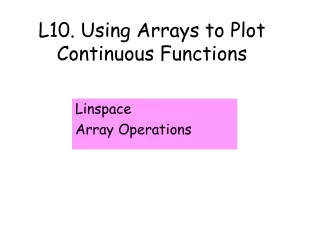
L10. Using Arrays to Plot Continuous Functions
390 likes | 412 Views
Learn how to use arrays and tables in MATLAB to plot continuous functions. Generate tables and plots based on different points and explore array operations. Examples provided.

L10. Using Arrays to Plot Continuous Functions
E N D
Presentation Transcript
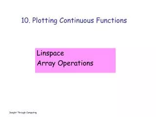
L10. Using Arrays to Plot Continuous Functions Linspace Array Operations
Table Plot x sin(x) 0.00 0.0 1.57 1.0 3.14 0.0 4.71 -1.0 6.28 0.0 Plot based on 5 points
Table Plot x sin(x) 0.000 0.000 0.784 0.707 1.571 1.000 2.357 0.707 3.142 0.000 3.927 -0.707 4.712 -1.000 5.498 -0.707 6.283 0.000 Plot based on 9 points
Table Plot Plot based on 200 points—looks smooth
Generating Tables and Plots x sin(x) 0.000 0.000 0.784 0.707 1.571 1.000 2.357 0.707 3.142 0.000 3.927 -0.707 4.712 -1.000 5.498 -0.707 6.283 0.000 x = linspace(0,2*pi,9); y = sin(x); plot(x,y)
linspace x = linspace(1,3,5) x : 1.0 1.5 2.0 2.5 3.0 “x is a table of values” “x is an array” “x is a vector”
linspace x = linspace(0,1,101) … x : 0.00 0.01 0.02 0.99 1.00
Linspace Syntax linspace( , , ) Left Endpoint Number of Points Right Endpoint
Built-In Functions Accept Arrays 0.00 1.57 3.14 4.71 6.28 sin x sin(x) 0.00 0.0 1.57 1.0 3.14 0.0 4.71 -1.0 6.28 0.0 And…
Return Array of Function-evals sin 0.00 1.00 0.00 -1.00 0.00 x sin(x) 0.00 0.0 1.57 1.0 3.14 0.0 4.71 -1.0 6.28 0.0
Examples x = linspace(0,1,200); y = exp(x); plot(x,y) x = linspace(1,10,200); y = log(x); plot(x,y)
Can We Plot This? -2 <= x <= 3
Can We Plot This? -2 <= x <= 3 Yes! x = linspace(-2,3,200); y = sin(5*x).*exp(-x/2)./(1 + x.^2) plot(x,y) Array operations
Must LearnHow to Operate on Arrays Look at four simpler plotting challenges.
Scale (*) a: -5 8 10 c = s*a s: 2 20 16 -10 c:
Addition a: -5 8 10 c = a + b b: 2 1 4 12 12 -4 c:
Subtraction a: -5 8 10 c = a - b b: 2 1 4 8 4 -6 c:
E.g.1 Sol’n x = linspace(0,4*pi,200); y1 = sin(x); y2 = cos(3*x); y3 = sin(20*x); y = 2*y1 - y2 + .1*y3; plot(x,y)
Exponentiation a: -5 8 10 c = a.^s s: 2 100 64 25 c: .^
Shift a: -5 8 10 c = a + s s: 2 12 10 -3 c:
Reciprocation a: -5 8 10 c = 1./a .1 .125 -.2 c:
E.g.2 Sol’n x = linspace(-5,5,200); y = 5./(1+ x.^2); plot(x,y)
Negation a: -5 8 10 c = -a -10 -8 5 c:
Scale (/) a: -5 8 10 c = a/s s: 2 5 4 -2.5 c:
Multiplication a: -5 8 10 c = a .* b b: 2 1 4 20 32 -5 c: .*
E.g.3 Sol’n x = linspace(0,3,200); y = exp(-x/2).*sin(10*x); plot(x,y)
Division a: -5 8 10 c = a ./ b b: 2 1 4 5 2 -5 c: ./
E.g.4 Sol’n x = linspace(-2*pi,2*pi,200); y = (.2*x.^3 - x)./(1.1 + cos(x)); plot(x,y)
Question Time How many errors in the following statement given that x = linspace(0,1,100): Y = (3*x .+ 1)/(1 + x^2) A. 0 B. 1 C. 2 D. 3 E. 4
Question Time How many errors in the following statement given that x = linspace(0,1,100): Y = (3*x .+ 1)/(1 + x^2) Y = (3*x + 1) ./ (1 + x.^2) A. 0 B. 1 C. 2 D. 3 E. 4
Question Time Does this assign to y the values sin(0o), sin(1o),…,sin(90o)? x = linspace(0,pi/2,90); y = sin(x); A. Yes B. No
Question Time Does this assign to y the values sin(0o), sin(1o),…,sin(90o)? %x = linspace(0,pi/2,90); x = linspace(0,pi/2,91); y = sin(x); A. Yes B. No
Plotting an Ellipse Better:
Solution a = input(‘Major semiaxis:’); b = input(‘Minor semiaxis:’); t = linspace(0,2*pi,200); x = a*cos(t); y = b*sin(t); plot(x,y) axis equal off