Data Storage Model for Environmental Monitoring Wireless Sensor Networks

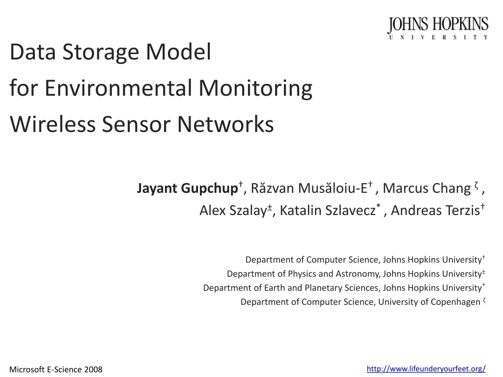
1. Data Storage Model for Environmental Monitoring Wireless Sensor Networks JayantGupchup†, RăzvanMusăloiu-E† , Marcus Chang ζ , Alex Szalay±, KatalinSzlavecz* , Andreas Terzis† Department of Computer Science, Johns Hopkins University† Department of Physics and Astronomy, Johns Hopkins University± Department of Earth and Planetary Sciences, Johns Hopkins University* Department of Computer Science, University of Copenhagen ζ

2. Outline • Life Under Your Feet • First Deployment(s) • Lessons Learned • System Architecture • Results • Discussion

3. Life Under Your Feet • Understand spatial and temporal heterogeneity of soil ecosystems • Correlate ecological data with environmental variables (E.g. Soil Temperature) • Why Wireless Sensor Networks? • Non Intrusive • Continuous collection of data • Data collection at varying scales • Reduction in labor • Built-in Intelligence

4. A Typical Sensor Network Stable Storage Gateway/ Basestation “MOTE” “Box” + “Sensors” …….

5. Previous Deployments

6. First Deployment - Olin • September 9, 2005 – July 21, 2006 • Location: Olin Hall JHU Campus (Urban Forest) • Goal: Proof of Concept Deployment • 10 Boxes • Soil Temperature • Soil Moisture • Box Temp • Light • Sampling Rate : 1 minute • Scientifically useful data • 1 Minute Sampling is overkill

7. Second Deployment – Leakin Park • March 3, 2006 – November 5, 2007 • Location: Leakin Park, Baltimore (urban forest) • Goal: Correlate data collected by Baltimore Ecosystem Study • 6 Boxes • Soil Temperature • Soil Moisture • Box Temp • Light • Sampling Rate : 20 minutes • Periodic data downloads are crucial

8. Third Deployment – Jug bay Turtle Monitoring • June 22, 2007– April 26, 2008 • Location: Jug bay Wetlands, Arundel Co. Md • Goal - Monitor: • nesting conditions • over-wintering conditions • 13 Boxes • Soil Temperature • Soil Moisture • Box Temp • Light

9. Lessons Learned

10. Schema Lessons • Hardware can fail! • Schema needs to handle hardware replacements from a science point of view • Sensor Heterogeneity • Inter Deployment • Intra Deployment • Seamless correlation of data • Across Deployments • Sensor Types

11. Data-Yield Lessons • Metadata is important • It can unlock many mysteries! • Save time, resources • Early Detection of Failure is crucial • Increase Data-Yield

12. Unified Architecture • Some details/tasks are deployment specific • Some details/tasks are deployment independent • 2-phase Loading • Phase I : Staging • Meta Information • Deployment Specific • Computer Scientists care about deployments details • Phase II : Science • Hardware Agnostic • Deployment Agnostic • Scientists interested in data (not deployments details)

13. Current Deployments

14. Olin Revisited • July 13, 2008 – n/a • Location: Olin Hall JHU Campus (Urban Forest) • Goal: Spatial & temporal variation of urban soil ecosystems • 19 Boxes • Soil Temperature • Soil Moisture • Box Temp • Box Humidity • Light • Multiple hardware Replacement Dynamics Boxes Known Locations

15. Cub Hill Deployment • July 13, 2008 – n/a • Location: Towson, MD • Co-located near a CO2 Flux tower • Goal: • Exchange of ambient CO2 , soil CO2 • Effect on Soil ecosystems • 31 Boxes • Soil CO2 • Soil Temperature • Soil Moisture • Box Temp • Box Humidity • Light • New Sensor Type

16. System Architecture 2 phase Loading • Every 6 hours • Journal of actions

17. 2 phase Loading & Health Monitoring

18. Stage DB - I • Downloads ingested in stage DB • Raw Data in the form of packets • Journal of Actions taken by the mote. • Each download acts as a “version number” • Origins of the data can be traced using the version number • Routines to undo corrupted downloads using version number • Stage DB contains tracking information • When was hardware replaced? • What hardware is at what locations? • What is the health level of the components

19. Stage DB - II • Wireless networking information • # of packet retransmissions • radio-on time • Last known contact time of each mote • Download Paths • # of reboots • # of beacons • Timestamp Reconstruction ….

20. Stage DB III (Timestamp Reconstruction) • Each mote runs a logical clock • Measurements are marked using local timestamps (LTS) • GTS = α * LTS + β • GTS is the global timestamp (unixts) • α is the clock drift • β is the start time • Periodically collect (LTS,GTS) pairs. “Anchor Points” • Fit (α, β) Slope (α ): Clock Skew β

21. Stage DB IV (Timestamp Reconstruction) • Motes reboot • Start new segments • Fit no longer applicable • Detect “new segments” • Obtain new anchor points • Compute new fits for the new segment • When no anchor points available? • Sundial: using sunlight to reconstruct global timestamps, to appear in proceedings of European wireless sensor networks (EWSN 2009) Segment

22. Science Database • Location centric • Data Series references using (Location, Type) • Hardware agnostic • Deployment agnostic • Unified Science Database • Correlate Heterogeneous data • Multiple deployments • Multiple Sensor Types • Multiple Scales Box Replacements

23. Results • 19 Boxes Replaced • 7 Due to High Moisture • 12 Due to Radio Failure & Misc. • 16 Sensors Replaced • Detected Lethal code bugs • Significantly reduce lifetime of the network • Detected failures early • Data continuity • Data Yield (fraction of usable data) is high • Scientists are happy

24. Visualize Data using SenseWeb Senseweb (http://atom.research.microsoft.com/sensewebv3/sensormap/) Search “Mount Calvert”

25. Life Under Your Feet Team • Acknowledgements: • Liqian Luo (Microsoft Research) • Chris Swarth (Jug bay Wetland Sanctuary) • Maryland Dept. of Forest Service

26. Extra

27. Summary • End-to-End Sensor Data • Deployment Specific : Stage • Deployment Independent : Science • Metadata crucial for provenance purposes • Early detection of Failures • Ensures high data-yield