Mastering Binary Decision Diagrams (BDD) for Boolean Functions
Learn about Ordered Binary Decision Diagrams (OBDDs), Binary Decision Trees (BDTs), Reduced Ordered BDDs (ROBDDs), and their applications in formal verification of systems. Explore ROBDD creation, canonical form property, variable ordering problem, and heuristics. Discover how to optimize variable ordering for efficient Boolean function representation.

Mastering Binary Decision Diagrams (BDD) for Boolean Functions
E N D
Presentation Transcript
NETW703 Network Protocols BDDs & Theorem Proving Binary Decision Diagrams Dr. Eng. Amr T. Abdel-Hamid • Lectures are based on slides by: • K. Havelund & Agroce, Reliable Software: Testing and Monitoring, CMU. • E. Clarke, Formal Methods, to be updated by course name • S. Tahar, E. Cerny and X. Song, “ Formal Verification of Systems”. Winter 2012
Binary Decision Diagrams • Ordered binary decision diagrams (OBDDs) are a canonical form for Boolean formulas. • OBDDs are often substantially more compact than traditional normal forms. • Moreover, they can be manipulated very efficiently. • Introduced at: • R. E. Bryant. Graph-based algorithms for boolean function manipulation. IEEE Transactions on Computers, C-35(8), 1986.
Binary Decision Trees • A Binary decision tree is a rooted, directed tree with two types of vertices, terminal vertices and nonterminal vertices. • Each nonterminal vertex v is labeled by a variable var(v) and has two successors: • low (v) corresponding to the case where the variable is assigned 0, and high (v) corresponding to the case where the variable is assigned 1. • Each terminal vertex v is labeled by value(v) which is either 0 or 1
Example • BDT for a two-bit comparator, f(a1,a2,b1,b2) = (a1 b1) (a2 b2)
Binary Decision Diagram • i.e. exactly like decision TREE
Reduced Ordered BDDs • In practical applications, it is desirable to have a canonical representation for Boolean functions. • This simplifies tasks like checking equivalence of two formulas and deciding if a given formula is satisfiable or not. • Such a representation must guarantee that two Boolean functions are logically equivalent if and • only if they have isomorphic representations.
Reduced Ordered BDD • Canonical Form property • A canonical representation for Boolean functions is desirable: • two Boolean functions are logically equivalent iff they have isomorphic representations • This simplifies checking equivalence of two formulas and deciding if a formula is satisfiable • Two BDDs are isomorphic if there exists a bijection h between the graphs such that • Terminals are mapped to terminals and nonterminals are mapped to nonterminals • For every terminal vertex v, value(v) = value(h(v)), and • For every nonterminal vertex v: var(v) = var(h(v)), h(low(v)) = low(h(v)), and h(high(v)) = high(h(v))
Canonical Form property • Bryant (1986) showed that BDDs are a canonical representation for Boolean functions under two restrictions: • the variables appear in the same order along each path from the root to a terminal • there are no isomorphic subtrees or redundant vertices
Reduced Ordered Binary Decision Diagrams (ROBDDs): CREATION • Canonical Form Property • Requirement (1): Impose total order “<” on the variables in the formula: if vertex u has a nonterminal successor v, then var(u) < var(v) • Requirement (2): repeatedly apply three transformation rules (or implicitly in operations such as disjunction or conjunction)
RoBDD Creation 1) Remove duplicate terminals: eliminate all but one terminal vertex with a given label and redirect all arcs to the eliminated vertices to the remaining one
RoBDD Creation 2. Remove duplicate nonterminals: if nonterminals u and v have var(u) = var(v), low(u) = low(v) and high(u) = high(v), eliminate one of the two vertices and redirect all incoming arcs to the other vertex
3. Remove redundant tests: if nonterminal vertex v has low(v) = high(v), eliminate v and redirect all incoming arcs to low(v)
ROBDD Example • Creating the ROBDD for (x⊕y⊕z)
Canonical Form Property (cont’d) • A canonical form is obtained by applying the transformation rules until no further application is possible • Bryant showed how this can be done by a procedure called Reduce in linear time • Applications: • checking equivalence: verify isomorphism between ROBDDs • non-satisfiability: verify if ROBDD has only one terminal node, labeled by 0 • tautology: verify if ROBDD has only one terminal node, labeled by 1
Variable Ordering Problem • The problem of finding the optimal variable order is NP-complete • Some Boolean functions have exponential size ROBDDs for any order (e.g., multiplier) • Heuristics for Variable Ordering • Heuristics developed for finding a good variable order (if it exists) • Intuition for these heuristics comes from the observation that ROBDDs tend to be smaller when related variables are close together in the order • Variables appearing in a subcircuit are related: they determine the subcircuit’s output should usually be close together in the order • Dynamic Variable Ordering • Useful if no obvious static ordering heuristic applies • During verification operations (e.g., reachability analysis) functions change, hence initial order is not good later on • Good ROBDD packages periodically internally reorder variables to reduce ROBDD size • Basic approach based on neighboring variable exchange • Among a number of trials the best is taken, and the exchange is repeated
Model Checking • The Good: • If it works, model checking (unlike theorem proving) is a push-button tool. • The Bad: • If the system is too large, model checking cannot be applied because of state explosion. • & The Ugly • The system (and/or property) then needs to be suitably “abstracted” in order to use model checking.
Approximate Model Checking • Representing exact state sets may involve large BDDs Compute approximations to reachable states • Potentially smaller representation • Over-approximation : • No bugs found Circuit verified correct • Bugs found may be real or false • Under-approximation : • Bug found Real bug • No bugs found Circuit may still contain bugs Buggy states Reachable states
Theorem Proving • Prove that an implementation satisfies a specification by mathematical reasoning • Implementation and specification expressed as formulas in a formal logic • Required relationship (logical equivalence/logical implication) described as a theorem to be proven within the context of a proof calculus • A proof system: • A set of axioms and inference rules (simplification, rewriting, induction, etc.)
Theorem Proving Idea • Properties specified in a Logical Language (SPEC) • System behavior also in the same language (DES) • Establish (DES -> SPEC) as a theorem. • A logical System: • Alanguage defining constants, functions and predicates • A no. of axioms expressing properties of the constants, function, types, etc. • Inference Rules • A Theorem • `follows' from axioms by application of inference rules has a proof
First-Order Logic • Propositional logic: reasoning about complete sentences. • First-order logic: also reasoning about individual objects and relationships between them. • Syntax • Objects (in FOL) are denoted by expressions called terms: • Constants a, b, c,... ; Variables u, v, w,... ; • f(t1, t2,..., tn) where t1, t2,..., tn are terms and f a function symbol of n arguments • Predicates: • true (T) and false (F) • p(t1, t2,..., tn) where t1, t2,..., tn are terms and p a predicate symbol of n arguments
First-Order Logic (cont.) • Formulas: • Predicates: • P and Q formulas, then P, P Q, P Q, P Q, P Q are formulas • x a variable, P a formula, then x.P, x.Q are formulas (x is not free in P, Q)
First-Order Logic (cont’d) • The Validity Problem of FOL • To decide the validity for formulas of FOL, the truth table method does not work! • Reason: must deal with structures not just truth assignments. • Structures need not be finite ... • Semi-decidable (partially solvable) • There is an algorithm which starts with an input, and • if the input is valid then it terminates after a finite number of steps, and outputs the correct value (Yes or No) • if the input is not valid then it reaches a reject halt or loops forever • Theorem (Church-Turing, 1936) The validity problem for formulas of FOL is undecidable, but semi-decidable. • Some subsets of FOL are decidable.
Higher-Order Logic • First-order logic: only domain variables can be quantified. • Second-order logic: quantification over subsets of variables (i.e., over predicates). • Higher-order logics: quantification over arbitrary predicates and functions. • Higher-Order Logic: • Variables can be functions and predicates, • Functions and predicates can take functions as arguments and return functions as values, • Quantification over functions and predicates. • Since arguments and results of predicates and functions can themselves be predicates or functions, this imparts a first-class status to functions, and allows them to be manipulated just like ordinary values
HOL • Example 1: (mathematical induction) • P. [P(0) (n. P(n) P(n+1))] n.P(n) (Impossible to express it in FOL) • Example 2: Function Rise defined as Rise (c, t) = c(t) c(t+1) • Rise expresses the notion that a signal c rises at time t.
Higher-Order Logic • Advantage: • high expressive power! • Disadvantages: • Incompleteness of a sound proof system for most higher-order logics • Theorem (Gödel, 1931) • “There is no complete deduction system for the second-order logic” • Inconsistencies can arise in higher-order systems if semantics not carefully defined • “Russell Paradox”: • Let P be defined by P(Q) = ¬Q(Q). • By substituting P for Q, leads to P(P) = ¬P(P),
Theorem Proving Systems • Some theorem proving systems: • Boyer-Moore (first-order logic) • HOL (higher-order logic) • PVS (higher-order logic) • Lambda (higher-order logic) From PVS website: “PVS is a large and complex system and it takes a long while to learn to use it effectively. You should be prepared to invest six months to become a moderately skilled user”
HOL • HOL (Higher-Order Logic) developed at University of Cambridge • Interactive environment (in ML, Meta Language) for machine assisted theorem proving in higherorder logic (a proof assistant) • Steps of a proof are implemented by applying inference rules chosen by the user; HOL checks that the steps are safe • All inferences rules are built on top of eight primitive inference rules • Mechanism to carry out backward proofs by applying built-in ML functions called tactics and tacticals • By building complex tactics, the user can customize proof strategies • Numerous applications in software and hardware verification
HOL • HOL provides considerable built-in theorem-proving infrastructure: • a powerful rewriting subsystems • library facility containing useful theories and tools for general use • Decision procedures for tautologies and semi-decision • procedure for linear arithmetic provided as libraries • The approach to mechanizing formal proof used in HOL is due to Robin Milner.
Proof Styles in HOL • Forward proof style: Goal-directed (or Backward) proof style:
Example 1: Logic AND • AND Specification: AND_SPEC (i1,i2,out) := out = i1 ∧ i2 • NAND specification: NAND (i1,i2,out) := out = ¬(i1 ∧ i2) • NOT specification: NOT (i, out) := out = ¬ I • AND Implementation: AND_IMPL (i1,i2,out) := ∃x. NAND (i1,i2,x) ∧ NOT (x,out)
Example 1: Logic AND • Proof Goal: ∀ i1, i2, out. AND_IMPL(i1,i2,out) ⇒ ANDSPEC(i1,i2,out) • Proof (forward) AND_IMP(i1,i2,out) {from above circuit diagram} ∃ x. NAND (i1,i2,x) ∧ NOT (x,out) {by def. of AND impl} NAND (i1,i2,x) ∧ NOT(x,out) {strip off “∃ x.”} NAND (i1,i2,x) {left conjunct of line 3} x =¬ (i1 ∧ i2) {by def. of NAND} NOT (x,out) {right conjunct of line 3} out = ¬ x {by def. of NOT} out = ¬(¬(i1 ∧ i2) {substitution, line 5 into 7} out =(i1 ∧ i2) {simplify, ¬¬ t=t} AND (i1,i2,out) {by def. of AND spec} AND_IMPL (i1,i2,out) ⇒ AND_SPEC (i1,i2,out) Q.E.D.
Inductive Proofs • Inductive Proofs Must Have: • Base Case (value): • where you prove it is true about the base case • Inductive Hypothesis (value): • where you state what will be assume in this proof • Inductive Step (value) • show: • where you state what will be proven below • proof: • where you prove what is stated in the show portion • this proof must use the Inductive Hypothesis sometime during the proof
Example 2 • Prove this statement: • Base Case (n=1): • Inductive Hypothesis (n=p): • Inductive Step (n=p+1): • Show:
Example 3 N-Bit Adder • Verification of Generic Circuits • used in datapath design and verification • idea: verify n-bit circuit then specialize proof for specific value of n, (i.e., once proven for n, a simple instantiation of the theorem for any concrete value, e.g. 32, gets a proven theorem for that instance). • use of induction proof • Specification • N-ADDER_SPEC (n,in1,in2,cin,sum,cout):= (in1 + in2 + cin = 2n+1 * cout + sum)
Example 3 N-Bit Adder • Implementation
Example 3 N-Bit Adder • Recursive Definition: N-ADDER_IMP(n,in1[0..n-1],in2[0..n-1],cin,sum[0..n-1],cout):= ∃ w. N-ADDER_IMP(n-1,in1[0..n-2],in2[0..n-2],cin,sum[0..n-2],w) ∧ N-ADDER_IMP(1,in1[n-1],in2[n-1],w,sum[n-1],cout) Notes: • N-ADDER_IMP(1,in1[i],in2[i],cin,sum[i],cout) = ADDER_IMP(in1[i],in2[i],cin,sum[i],cout) • Data abstraction function (vn: bitvec → nat) to relate bit vectors to natural numbers: • vn(x[0]):= bn(x[0]) • vn(x[0,n]):= 2n * bn(x[n]) + vn(x[0,n-1]
Example 3 N-Bit Adder • Proof goal: ∀ n, in1, in2, cin, sum, cout. N-ADDER_IMP(n,in1[0..n-1],in2[0..n-1],cin,sum[0..n-1],cout) ⇒ N-ADDER_SPEC(n, vn(in1[0..n-1]), vn(in2[0..n-1]), vn(cin), vn(sum[0..n-1]), vn(cout)) • As an example can be instantiated with n = 32: ∀ in1, in2, cin, sum, cout. N-ADDER_IMP(in1[0..31],in2[0..31],cin,sum[0..31],cout) ⇒ N-ADDER_SPEC(vn(in1[0..31]), vn(in2[0..31]), vn(cin), vn(sum[0..31]), vn(cout))
Example 3 N-Bit Adder • Proof by induction over n: • basis step: N-ADDER_IMP(1,in1[0],in2[0],cin,sum[0],cout) ⇒ N-ADDER_SPEC(1,vn(in1[0]),vn(in2[0]),vn(cin),vn(sum[0]),vn(cout)) • Induction Step: [N-ADDER_IMP(n,in1[0..n-1],in2[0..n-1],cin,sum[0..n-1],cout) ⇒ N-ADDER_SPEC(n,vn(in1[0..n-1]),vn(in2[0..n-1]),vn(cin),vn(sum[0..n-1]),vn(cout)) ] ⇒ [N-ADDER_IMP(n+1,in1[0..n],in2[0..n],cin,sum[0..n],cout) ⇒ N-ADDER_SPEC(n+1,vn(in1[0..n]),vn(in2[0..n]),vn(cin),vn(sum[0..n]),vn(cout))]
Conclusions • Advantages of Theorem Proving • High abstraction and expressive notation • Powerful logic and reasoning, e.g., induction • Can exploit hierarchy and regularity, puts user in control • Can be customized with tactics (programs that build larger proofs steps from basic ones) • Useful for specifying and verifying parameterized (generic) datapath-dominated designs • Unrestricted applications (at least theoretically) • Limitations of Theorem Proving: • Interactive (under user guidance): use many lemmas, large numbers of commands • Large human investment to prove small theorems • Usable only by experts: difficult to prove large / hard theorems • Requires deep understanding of the both the design and HOL (while-box verification) • must develop proficiency in proving by working on simple but similar problems.
We are not alone Theorem proving Model checking Testing
Hybrid Verification • Formal Verification using • Theorem Proving + Model Checking Model Checking Theorem Proving
Hybrid Verification ……. G1 G2 G3 Gn G1’’ G2’’ G3’’ Gn’’ |-Goal Imp. Spec. |-Goal Imp.(x y ….) Spec.((y= ..) (…..)) G2’ G3’ G1’ Gn’ Use model checking to verify Sub-Goals
Different Verification Methods • Testing (Simulation/Emulation) • Theorem Proving • Model checking (automatic verification) Testing Theorem Proving Model Checking
Semi-formal Verification Simulation Monitor Simulation Driver Simulation Engine Symbolic Simulation Conventional Diagnosis of Unverified Portions Coverage Analysis Guided vector generation Extension Devadas and Keutzer’s proposal: A pragmatic suggestion for SOC verification
Semi-formal Verification • Smart simulation: • Use properties to generate directed test vectors. • Maximize chances of detecting bugs at small cost • Coverage metrics crucial? • Use metrics to determine • Unexercised parts of design: Guide vector generation • Adequacy of verification: When to stop?
Did you find the BUG yet? • Verification and testing problem is an open question with multi-Billion $ Research per year. • A great Masters Research Topic
A Final Proof • Software engineers want to be real engineers. • Real engineers use mathematics. • Formal methods are the mathematics of software engineering. • Therefore, software engineers should use formal methods. Mike Holloway, NASA