
Dynamic Vector Field Visualization with Parameterized Arrows
This project presents a dynamic visualization of a vector field defined by the parameters 'a' and 'b'. The vectors are governed by the equations: x-derivative as -x + a*y + x^2*y and y-derivative as b - a*y - x^2*y. With 20 points distributed within a specified window, this visualization helps to analyze how changes in the parameters affect the overall behavior of the system. Interactive elements allow for adjustment of parameters, offering insight into the complexities of two-dimensional vector fields.

Dynamic Vector Field Visualization with Parameterized Arrows
E N D
Presentation Transcript
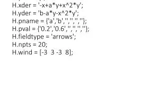
%% PPLANE file %% H.name = 'glicp.pps'; H.xvar = 'x'; H.yvar = 'y'; H.xder = '-x+a*y+x^2*y'; H.yder = 'b-a*y-x^2*y'; H.pname = {'a','b','','','',''}; H.pval = {'0.2','0.6','','','',''}; H.fieldtype = 'arrows'; H.npts = 20; H.wind = [-3 3 -3 8];