Download
1 / 46
490 likes | 635 Views
Chapter 7 Estimating Population Values. Chapter Goals. After completing this chapter, you should be able to: Distinguish between a point estimate and a confidence interval estimate

E N D
Chapter Goals After completing this chapter, you should be able to: • Distinguish between a point estimate and a confidence interval estimate • Construct and interpret a confidence interval estimate for a single population mean using both the z and t distributions • Determine the required sample size to estimate a single population mean within a specified margin of error • Form and interpret a confidence interval estimate for a single population proportion
Confidence Intervals Content of this chapter • Confidence Intervals for the Population Mean, μ when Population Standard Deviation σ is Known • when Population Standard Deviation σ is Unknown • Determining the Required Sample Size • Confidence Intervals for the Population Proportion, p
Point and Interval Estimates • A point estimate is a single number, • a confidence interval provides additional information about variability Upper Confidence Limit Lower Confidence Limit Point Estimate Width of confidence interval
Point Estimates We can estimate a Population Parameter … with a SampleStatistic (a Point Estimate) μ x Mean p Proportion p
Confidence Intervals • How much uncertainty is associated with a point estimate of a population parameter? • An interval estimate provides more information about a population characteristic than does a point estimate • Such interval estimates are called confidence intervals
Confidence Interval Estimate • An interval gives a range of values: • Takes into consideration variation in sample statistics from sample to sample • Based on observation from 1 sample • Gives information about closeness to unknown population parameters • Stated in terms of level of confidence • Never 100% sure
I am 95% confident that μ is between 40 & 60. Estimation Process Random Sample Population Mean x = 50 (mean, μ, is unknown) Sample
General Formula • The general formula for all confidence intervals is: Point Estimate (Critical Value)(Standard Error)
Confidence Level • Confidence Level • Confidence in which the interval will contain the unknown population parameter • A percentage (less than 100%)
Confidence Level, (1-) (continued) • Suppose confidence level = 95% • Also written (1 - ) = .95 • A relative frequency interpretation: • In the long run, 95% of all the confidence intervals that can be constructed will contain the unknown true parameter • A specific interval either will contain or will not contain the true parameter • No probability involved in a specific interval
Confidence Intervals Confidence Intervals Population Mean Population Proportion σKnown σUnknown
Confidence Interval for μ(σ Known) • Assumptions • Population standard deviation σis known • Population is normally distributed • If population is not normal, use large sample • Confidence interval estimate
Finding the Critical Value • Consider a 95% confidence interval: z.025= -1.96 z.025= 1.96 z units: 0 Lower Confidence Limit Upper Confidence Limit x units: Point Estimate Point Estimate
Common Levels of Confidence • Commonly used confidence levels are 90%, 95%, and 99% Confidence Coefficient, Confidence Level z value, 80% 90% 95% 98% 99% 99.8% 99.9% .80 .90 .95 .98 .99 .998 .999 1.28 1.645 1.96 2.33 2.57 3.08 3.27
Interval and Level of Confidence Sampling Distribution of the Mean x Intervals extend from to x1 100(1-)%of intervals constructed contain μ; 100% do not. x2 Confidence Intervals
Margin of Error • Margin of Error (e): the amount added and subtracted to the point estimate to form the confidence interval Example: Margin of error for estimating μ, σ known:
Factors Affecting Margin of Error • Data variation, σ : e as σ • Sample size, n : e as n • Level of confidence, 1 - : e if 1 -
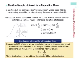
Example • A sample of 11 circuits from a large normal population has a mean resistance of 2.20 ohms. We know from past testing that the population standard deviation is .35 ohms. • Determine a 95% confidence interval for the true mean resistance of the population.
Example (continued) • A sample of 11 circuits from a large normal population has a mean resistance of 2.20 ohms. We know from past testing that the population standard deviation is .35 ohms. • Solution:
Interpretation • We are 95% confident that the true mean resistance is between 1.9932 and 2.4068 ohms • Although the true mean may or may not be in this interval, 95% of intervals formed in this manner will contain the true mean • An incorrect interpretation is that there is 95% probability that this interval contains the true population mean. (This interval either does or does not contain the true mean, there is no probability for a single interval)
Confidence Intervals Confidence Intervals Population Mean Population Proportion σKnown σUnknown
Confidence Interval for μ(σ Unknown) • If the population standard deviation σ is unknown, we can substitute the sample standard deviation, s • This introduces extra uncertainty, since s is variable from sample to sample • So we use the t distribution instead of the normal distribution
Confidence Interval for μ(σ Unknown) (continued) • Assumptions • Population standard deviation is unknown • Population is normally distributed • If population is not normal, use large sample • Use Student’s t Distribution • Confidence Interval Estimate
Student’s t Distribution • The t is a family of distributions • The t value depends on degrees of freedom (d.f.) • Number of observations that are free to vary after sample mean has been calculated d.f. = n - 1
Degrees of Freedom (df) Idea: Number of observations that are free to vary after sample mean has been calculated Example:Suppose the mean of 3 numbers is 8.0 Let x1 = 7 Let x2 = 8 What is x3? If the mean of these three values is 8.0, then x3must be 9 (i.e., x3 is not free to vary) Here, n = 3, so degrees of freedom = n -1 = 3 – 1 = 2 (2 values can be any numbers, but the third is not free to vary for a given mean)
Student’s t Distribution Note: t z as n increases Standard Normal (t with df = ) t (df = 13) t-distributions are bell-shaped and symmetric, but have ‘fatter’ tails than the normal t (df = 5) t 0
Student’s t Table Upper Tail Area Let: n = 3 df = n - 1 = 2= .10/2 =.05 df .25 .10 .05 1 1.000 3.078 6.314 0.817 1.886 2 2.920 /2 = .05 3 0.765 1.638 2.353 The body of the table contains t values, not probabilities 0 t 2.920
t distribution values With comparison to the z value Confidence t t t z Level (10 d.f.)(20 d.f.)(30 d.f.) ____ .80 1.372 1.325 1.310 1.28 .90 1.812 1.725 1.697 1.64 .95 2.228 2.086 2.042 1.96 .99 3.169 2.845 2.750 2.57 Note: t z as n increases
Example A random sample of n = 25 has x = 50 and s = 8. Form a 95% confidence interval for μ • d.f. = n – 1 = 24, so The confidence interval is 46.698 …………….. 53.302
Approximation for Large Samples • Since t approaches z as the sample size increases, an approximation is sometimes used when n 30: Technically correct Approximation for large n
Determining Sample Size • The required sample size can be found to reach a desired margin of error (e) and level of confidence (1 -) • Required sample size, σ known:
Required Sample Size Example If = 45, what sample size is needed to be 90% confident of being correct within ± 5? So the required sample size is n = 220 (Always round up)
If σ is unknown • If unknown, σ can be estimated when using the required sample size formula • Use a value for σ that is expected to be at least as large as the true σ • Select a pilot sample and estimate σ with the sample standard deviation, s
Confidence Intervals Confidence Intervals Population Mean Population Proportion σKnown σUnknown
Confidence Intervals for the Population Proportion, p • An interval estimate for the population proportion ( p ) can be calculated by adding an allowance for uncertainty to the sample proportion ( p )
Confidence Intervals for the Population Proportion, p (continued) • Recall that the distribution of the sample proportion is approximately normal if the sample size is large, with standard deviation • We will estimate this with sample data:
Confidence interval endpoints • Upper and lower confidence limits for the population proportion are calculated with the formula • where • z is the standard normal value for the level of confidence desired • p is the sample proportion • n is the sample size
Example • A random sample of 100 people shows that 25 are left-handed. • Form a 95% confidence interval for the true proportion of left-handers
Example (continued) • A random sample of 100 people shows that 25 are left-handed. Form a 95% confidence interval for the true proportion of left-handers. 1. 2. 3.
Interpretation • We are 95% confident that the true percentage of left-handers in the population is between 16.51% and 33.49%. • Although this range may or may not contain the true proportion, 95% of intervals formed from samples of size 100 in this manner will contain the true proportion.
Changing the sample size • Increases in the sample size reduce the width of the confidence interval. Example: • If the sample size in the above example is doubled to 200, and if 50 are left-handed in the sample, then the interval is still centered at .25, but the width shrinks to .19 …… .31
Finding the Required Sample Size for proportion problems Define the margin of error: Solve for n: p can be estimated with a pilot sample, if necessary (or conservatively use p = .50)
What sample size...? • How large a sample would be necessary to estimate the true proportion defective in a large population within 3%,with 95% confidence? (Assume a pilot sample yields p = .12)
What sample size...? (continued) Solution: For 95% confidence, use Z = 1.96 E = .03 p = .12, so use this to estimate p So use n = 451
Chapter Summary • Illustrated estimation process • Discussed point estimates • Introduced interval estimates • Discussed confidence interval estimation for the mean (σ known) • Addressed determining sample size • Discussed confidence interval estimation for the mean (σ unknown) • Discussed confidence interval estimation for the proportion