Download
1 / 35
350 likes | 442 Views
This guide provides detailed information on how to bring images collected with different methods and at different times into spatial alignment using the AFNI software. Learn about the voxel-by-voxel comparison, reducing artifacts due to subject movements, and aligning functional time series data. Explore the algorithmic choices, interpolation methods, and parameters adjustment techniques for optimal image registration. Discover the programs like 3dvolreg and 2dImReg for aligning 3D volumes and 2D slices, respectively. Gain insights into intra-session registration examples and hybrid registration methods.

E N D
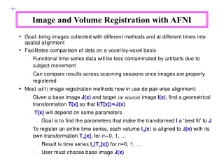
Image and Volume Registration with AFNI • Goal: bring images collected with different methods and at different times into spatial alignment • Facilitates comparison of data on a voxel-by-voxel basis • Functional time series data will be less contaminated by artifacts due to subject movement • Can compare results across scanning sessions once images are properly registered • Most (all?) image registration methods now in use do pair-wise alignment: • Given a base image J(x) and target (or source) image I(x), find a geometrical transformation T[x] so that I(T[x])≈J(x) • T[x] will depend on some parameters • Goal is to find the parameters that make the transformed I a ‘best fit’ to J • To register an entire time series, each volume In(x) is aligned to J(x) with its own transformation Tn[x], for n=0, 1, … • Result is time series In(Tn[x]) for n=0, 1, … • User must choose base image J(x)
Most image registration methods make 3 algorithmic choices: • How to measure mismatch E (for error) between I(T[x]) and J(x)? • Or … How to measure goodness of fit between I(T[x]) and J(x)? • E(parameters) –Goodness(parameters) • How to adjust parameters of T[x] to minimize E? • How to interpolate I(T[x]) to the J(x) grid? • So can compare voxel intensities directly • AFNI 3dvolreg program matches images by grayscale (intensity) values • E = (weighted) sum of squares differences = x w(x) · {I(T[x]) - J(x)}2 • Only useful for registering ‘like images’: • Good for SPGRSPGR, EPIEPI, but not good for SPGREPI • Parameters in T[x] are adjusted by “gradient descent” • Fast, but customized for the least squares E • Several interpolation methods are available: • Default method is Fourier interpolation • Polynomials of order 1, 3, 5, 7 (linear, cubic, quintic, and heptic) • This program is designed to run very fast for EPIEPI registration with small movements — good for FMRI purposes • Newer program 3dAllineate uses more complicated definitions of E • Will discuss this software later in the presentation
AFNI program 3dvolreg is for aligning 3D volumes by rigid movements • T[x] has 6 parameters: • Shifts along x-, y-, and z-axes; Rotations about x-, y-, and z-axes • Generically useful for intra- and inter-session alignment • Motions that occur within a single TR (2-3 s) cannot be corrected this way, since method assumes rigid movement of the entire volume • AFNI program 2dImReg is for aligning 2D slices • T[x] has 3 parameters for each slice in volume: • Shift along x-, y-axes; Rotation about z-axis • No out of slice plane shifts or rotations! • Useful for sagittal EPI scans where dominant subject movement is ‘nodding’ motion that may be faster than TR • It is possible and sometimes even useful to run 2dImReg to clean up sagittal nodding motion, followed by 3dvolreg to deal with out-of-slice motion • Hybrid ‘slice-into-volume’ registration: • Put each separate 2D image slice into the target volume with its own 6 movement parameters (3 out-of-plane as well as 3 in-plane) • Has been attempted, but the results are not much better than volume registration; method often fails on slices near edge of brain • We do not have a program to do this
Intra-session registration example: 3dvolreg -base 4 -heptic -zpad 4 \ -prefix fred1_epi_vr \ -1Dfile fred1_vr_dfile.1D \ fred1_epi+orig • -base 4 Selects sub-brick #4 of dataset fred1_epi+orig as base image J(x) • -heptic Use 7th order polynomial interpolation (my personal favorite) • -zpad 4 Pad each target image, I(x), with layers of zero voxels 4 deep on each face prior to shift/rotation, then strip them off afterwards (before output) • Zero padding is particularly desirable for -Fourier interpolation • Is also good to use for polynomial methods, since if there are large rotations, some data may get ‘lost’ when no zero padding if used (due to the 4-way shift algorithm used for very fast rotation of 3D volume data) • -prefix fred1_epi_vr Save output dataset into a new dataset with the given prefix name (e.g., fred1_epi_vr+orig) • -1Dfile fred1_vr_dfile.1D Save estimated movement parameters into a 1D (i.e., text) file with the given name • Movement parameters can be plotted with command 1dplot -volreg -dx 5 -xlabel Time fred1_vr_dfile.1D Input dataset name
Note motion peaks at time160s: subject jerked head up at that time • Can now register second dataset from same session: 3dvolreg -base ‘fred1_epi+orig[4]’ -heptic -zpad 4 \ -prefix fred2_epi_vr -1Dfile fred2_vr_dfile.1D \ fred2_epi+orig • Note base is from different dataset (fred1_epi+orig) than input (fred2_epi+orig) • Aligning all EPI volumes from session to EPI closest in time to SPGR • 1dplot -volreg -dx 5 -xlabel Time fred2_vr_dfile.1D
Graphs of a single voxel time series near the edge of the brain: • Top = slice-wise alignment • Middle = volume-wise adjustment • Bottom = no alignment • For this example, 2dImReg appears to produce better results. This is because most of the motion is ‘head nodding’ and the acquisition is sagittal • You should also use AFNI to scroll through the images (using the Index control) during the period of pronounced movement • Helps see if registration fixed problems • Examination of time series fred2_epi+orig and fred2_epi_vr_+orig shows that head movement up and down happened within about 1 TR interval • Assumption of rigid motion of 3D volumes is not good for this case • Can do 2D slice-wise registration with command 2dImReg -input fred2_epi+orig \ -basefile fred1_epi+orig \ -base 4 -prefix fred2_epi_2Dreg fred1_epi registered with 2dImReg fred1_epi registered with 3dvolreg fred1_epi unregistered
to3d defines defines relationship between EPI and SPGR in each session • 3dvolreg computes relationship between sessions • So can transform EPI from session 2 to orientation of session 1 • Issues in inter-session registration: • Subject’s head will be positioned differently (in orientation and location) • xyz-coordinates and anatomy don’t correspond • Anatomical coverage of EPI slices will differ between sessions • Geometrical relation between EPI and SPGR differs between session • Slice thickness may vary between sessions (try not to do this, OK?) • Intra-subject, inter-session registration (for multi-day studies on same subject) • Longitudinal or learning studies; re-use of cortical surface models • Transformation between sessions is calculated by registering high-resolution anatomicals from each session
At acquisition: Day 2 is rotated relative to Day 1 • After rotation to same orientation, then clipping to Day 2 xyz-grid • Anatomical coverage differs
Another problem: rotation occurs around center of individual datasets
Solutions to these problems: • Add appropriate shift to E2 on top of rotation • Allow for xyz shifts between days (E1-E2), and center shifts between EPI and SPGR (E1-S1 and E2-S2) • Pad EPI datasets with extra slices of zeros so that aligned datasets can fully contain all data from all sessions • Zero padding of a dataset can be done in to3d (at dataset creation time), or later using 3dZeropad • 3dvolreg and 3drotate can zero pad to make the output match a “grid parent” dataset in size and location
-twopass allows for larger motions • Recipe for intra-subject S2-to-S1 transformation: • Compute S2-to-S1 transformation: 3dvolreg -twopass -zpad 4 -base S1+orig\-prefix S2reg S2+orig • Rotation/shift parameters are saved in S2reg+orig.HEAD • If not done before (e.g., in to3d), zero pad E1 datasets: 3dZeropad -z 4 -prefix E1pad E1+orig • Register E1 datasets within the session: 3dvolreg -base ‘E1pad+orig[4]’ -prefix E1reg \ E1pad+orig • Register E2 datasets within the session, at the same time executing larger rotation/shift to session 1 coordinates that were saved in S2reg+orig.HEAD: 3dvolreg -base ‘E2+orig[4]’ \ -rotparent S2reg+orig \ -gridparent E1reg+orig \ -prefix E2reg E2reg+orig • -rotparent tells where the inter-session transformation comes from • -gridparent defines the output grid location/size of new dataset • Output dataset will be shifted and zero padded as needed to lie on top of E1reg+orig • These options put the aligned • E2reg into the same coordinates and grid as E1reg
Recipe above does not address problem of having different slice thickness in datasets of the same type (EPI and/or SPGR) in different sessions • Best solution: pay attention when you are scanning, and always use the same slice thickness for the same type of image • OK solution: use 3dZregrid to linearly interpolate datasets to a new slice thickness • Recipe above does not address issues of slice-dependent time offsets stored in data header from to3d(e.g., ‘alt+z’) • After interpolation to a rotated grid, voxel values can no longer be said to come from a particular time offset, since data from different slices will have been combined • Before doing this spatial interpolation, it makes sense to time-shift dataset to a common temporal origin • Time shifting can be done with program 3dTshift • Or by using the -tshift option in 3dvolreg, which first does the time shift to a common temporal origin, then does the 3D spatial registration • Further reading at the AFNI web site • File README.registration(plain text) has more detailed instructions and explanations about usage of 3dvolreg • File regnotes.pdf has some background information on issues and methods used in FMRI registration packages
Real-Time 3D Image Registration • The image alignment method using in 3dvolreg is also built into the AFNI real-time image acquisition plugin • Invoke by command afni -rt • Then use Define DatamodePluginsRT Options to control the operation of real-time (RT) image acquisition • Images (2D or 3D arrays of numbers) can be sent into AFNI through a TCP/IP socket • See the program rtfeedme.cfor sample of how to connect to AFNI and send the data • Also see file README.realtime for lots of details • 2D images will be assembled into 3D volumes = AFNI sub-bricks • Real-time plugin can also do 3D registration when each 3D volume is finished, and graph the movement parameters in real-time • Useful for seeing if the subject in the scanner is moving his head too much • If you see too much movement, telling the subject will usually help
Screen capture from example of real-time image acquisition and registration • Images and time series graphs can be viewed as data comes in • Graphs of movement parameters
New Program: 3dAllineate • 3dAllineate can be used align images from different methods • For example, to align EPI data to SPGR / MPRAGE: • Run 3dSkullStrip on the SPGR dataset so that it will be more like the EPI dataset (which will have the skull fat suppressed) • Use 3dAllineate to align the EPI volume(s) to the skull-stripped SPGR volume • Only works well if the EPI volume covers most of the brain • Program is slower than 3dvolreg • Allows more general spatial transformations • At present, 12 parameter affine: T[x] = Ax+b • Uses a more general-purpose optimization library than gradient descent • The NEWUOA package from Michael Powell at Oxford • Less efficient than a customized gradient descent formulation • But can be used in more situations • And is easier to put in the computer program, since there is no need to compute the derivatives of the cost function E
3dAllineate has several different “cost” functions (E) available • leastsq = Least Squares (like 3dvolreg) • mutualinfo = Mutual Information • norm_mutualinfo = Normalized Mutual Information • hellinger = Hellinger Metric [the default cost function] • corrratio_mul = Correlation ratio (symmetrized by multiplication) • corratio_add = Correlation ratio (symmetrized by addition) • corratio_uns = Correlation ratio (unsymmetric) • All cost functions, except “leastsq ”, are based on the joint histogram between images I(T[x]) and J(x) • The goal is to make I(T[x]) “predictable” as possible given J(x), as the parameters that define T[x] are varied • The different cost functions use different ideas of “predictable” • Perfect predictability = knowing value of J, can calculate value of I exactly • Least squares: I = J+ for some constants and • Joint histogram of I and J is “simple” in the idealized case of perfect predictability
I I I } } } J J J • J not useful in • predicting I • I can be accurately • predicted from J with • a linear formula: • -leastsq is OK • I can be accurately • predicted from J, but • nonlinearly: • -leastsq is BAD • Histogram cartoons:
} • Before alignment } • After alignment • (using -mutualinfo) • Actual histograms from a registration example • J(x) = 3dSkullStrip-ed MPRAGE I(x) = EPI volume I I J J
} • Before alignment } • After alignment • (using -mutualinfo) • grayscale underlay = J(x) = 3dSkullStrip-ed MPRAGE • color overlay = I(x) = EPI volume
Other 3dAllineate capabilities: • Save transformation parameters with option -1Dfile in one program run • Re-use them in a second program run on another input dataset with option -1Dapply • Interpolation: linear (polynomial order=1) during alignment • To produce output dataset: polynomials of order 1, 3, or 5 • Algorithm details: • Initial alignment starting with many sets of transformation parameters, using only a limited number of points from smoothed images • The best (smallest E) sets of parameters are further refined using more points from the images and less blurring • This continues until the final stage, where many points from the images and no blurring is used
The future for 3dAllineate: • Allow alignment to use manually placed control points (on both images)andthe image data • Will be useful for aligning highly distorted images or images with severe shading • Current AFNI program 3dTagalign allows registration with control points only • Nonlinear spatial transformations • For correcting distortions of EPI (relative to MPRAGE or SPGR) due to magnetic field inhomogeneity • For improving inter-subject brain alignment (Talairach) • Investigate the use of local computations of E(in a set of overlapping regions covering the images) and using the sum of these local E’s as the cost function • May be useful when relationship between I and J image intensities is spatially dependent • RF shading and/or Differing MRI contrasts • Save warp parameters in dataset headers for re-use
Algorithmic Features • Uses Powell’s NEWUOA software for minimization of general cost function • Lengthy search for initial transform parameters if two passes of registration are turned on [which is the default] • Random and grid search through hundreds of parameter sets for 15 good (low cost) parameter sets • Optimize a little bit from each ‘good’ set, using blurred images • Blurring the images means that small details won’t prevent a match • Keep best 4 of these parameter sets, and optimize them some more [keeping 4 sets is the default for -twobestoption] • Amount of blurring is reduced in several stages, followed by re-optimization of the transformation parameter sets on these less blurred images • -twofirst does this for first sub-brick, then uses the best parameter sets from the first sub-brick as the starting point for the rest of the sub-bricks [the default] • Use best 1 of these parameter sets as starting point for fine (un-blurred) parameter optimization • The slowest part of the program
Algorithmic Features • Goal is to find parameter set w such that E[ J(x) , I(T(x,w)) ] is small • T(x,w) = spatial transformation of x given w • J() = base image, I() = target image, E[] = cost function • For each x in base image space, compute T(x,w) and then interpolate I() at those points • For speed, program doesn’t use all points in J(), just a scattered collection of them, selected from an automatically generated mask • Mask can be turned off with -noauto option • At early stages, only a small collection of points [default=23456] is used when computing E[] • At later stages, more points are used, for higher accuracy • Recall that each stage is less blurred than the previous stages • Large fraction of CPU time is spent in interpolation of image I() over the collection of points used to compute E[]
Cost Functions • Except for least squares (actually,ls minimizes E=1.0–Pearson correlation coefficient), all cost functions are computed from 2D joint histogram of J(x) and I(T(x,w)) • Start and final histograms can be saved using hidden option-savehist Before After Source image Source image = rotated copy of Base image Base image
Histogram Based Cost Functions • Goal is to make 2D histogram become ‘simple’ in some sense, as a measurement of ‘predictability’ between J(x) and I(T(x,w)) • Entropy H() of a histogram (finite number of bins): • {pi} = probabilities of index i occuring • H({pi}) = –i pi log2(pi) > 0 • H({pi}) = Number of bits needed to encode a single value randomly drawn from the probabilities {pi} • Smaller entropy H means the values are ‘simpler’ to encode • Largest H is for uniform histogram (all pi equal)
Mutual Information • Entropy of 2D histogram • H({rij}) = –ij rij log2(rij) • Number of bits needed to encode value pairs (i,j) • Mutual Information between two distributions • Marginal (1D) histograms {pi} and {qj} • MI = H({pi}) + H({qj}) - H({rij}) • Number of bits required to encode 2 values separately minus number of bits required to encode them together (as a pair) • If 2D histogram is independent (rij= piqj) then MI = 0 = no gain from joint encoding • 3dAllineate minimizes E[J,I] = –MI(J,I) with -cost mi
Normalized MI • NMI = H({rij}) [ H({pi}) + H({qj}) ] • Ratio of number of bits to encode value pair divided by number of bits to encode two values separately • Minimize NMI with -cost nmi • Some say NMI is more robust for registration than MI, since MI can be large when there is no overlap between the two images NO overlap BAD overlap 100% overlap
Hellinger Metric • MI can be thought of as measuring a ‘distance’ between two 2D histograms: the joint distribution {rij} and the product distribution {piqj} • MI is not a ‘true’ distance: it doesn’t satisfy triangle inequality d(a,b)+d(b,c) > d(a,c) • Hellinger metric is a true distance in distribution “space”: • HM = ij [ rij– (piqj) ]2 • 3dAllineate minimizes –HM with -cost hel • This is the default cost function b c a
y x Correlation Ratio • Given 2 (non-independent) random variables x and y • Exp[y|x] is the expected value (mean) of y for a fixed value of x • Exp[a|b] Average value of ‘a’, given value of ‘b’ • Var(y|x) is the variance of y when x is fixed = amount of uncertainty about value of y when we know x • v(x)Var(y|x) is a function of x only • CR(x,y) 1 – Exp[v(x)]Var(y) • Relative reduction in uncertainty about value of y when x is known; large CR means Exp[y|x] is a good prediction of the value of y given the value of x • Does not say that Exp[x|y] is a good prediction of the x given y • CR(x,y) is a generalization of the Pearson correlation coefficient, which assumes that Exp[y|x] = x+
3dAllineate’s Symmetrical CR • First attempt to use CR in 3dAllineate didn’t give good results • Note asymmetry: CR(x,y) CR(y,x) • 3dAllineate now offers two different symmetric CR cost functions: • Compute both unsymmetric CR(x,y) and CR(y,x), then combine by Multiplying or Adding: • CRm(x,y) = 1 – [ Exp(v(x))Exp(v(y)) ][Var(y) Var(x) ] = CR(x,y)+CR(y,x) – CR(x,y) CR(y,x) • CRa(x,y) = 1 – 1/2 [Exp(v(x)) Var(y) ] –1/2 [Exp(v(y)) Var(x) ] = [ CR(x,y)+CR(y,x)]2 • These work better than CR(J,I) in my test problems • If Exp[y|x] can be used to predict y and/or Exp[x|y] can be used to predict x, then crM(x,y) will be large (close to 1) • 3dAllineate minimizes 1–CRm(J,I) with option -cost crM • 3dAllineate minimizes 1–CRa(J,I) with option -cost crA • 3dAllineate minimizes 1–CR(J,I) with option -cost crU
Test: Monkey EPI - Anat 6 DOF CRm 6 DOF NMI
Test: Monkey EPI - Anat 6 DOF HEL 6 DOF MI
Test: Monkey EPI - Anat 11 DOF CRm 11 DOF NMI
Test: Monkey EPI - Anat 11 DOF HEL 11 DOF MI