Image Pyramids and Blending
440 likes | 641 Views
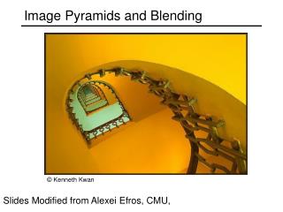
Image Pyramids and Blending. © Kenneth Kwan . Slides Modified from Alexei Efros, CMU, . Image Pyramids. Known as a Gaussian Pyramid [Burt and Adelson, 1983] In computer graphics, a mip map [Williams, 1983] A precursor to wavelet transform.

Image Pyramids and Blending
E N D
Presentation Transcript
Image Pyramids and Blending © Kenneth Kwan Slides Modified from Alexei Efros, CMU,
Image Pyramids • Known as a Gaussian Pyramid [Burt and Adelson, 1983] • In computer graphics, a mip map [Williams, 1983] • A precursor to wavelet transform
A bar in the big images is a hair on the zebra’s nose; in smaller images, a stripe; in the smallest, the animal’s nose Figure from David Forsyth
Gaussian Pyramid for encoding [Burt & Adelson, 1983] Prediction using weighted local Gaussian average Encode the difference as the Laplacian Both Laplacian and the Averaged image is easy to encode
Image sub-sampling 1/8 1/4 • Throw away every other row and column to create a 1/2 size image • - called image sub-sampling
Image sub-sampling 1/2 1/4 (2x zoom) 1/8 (4x zoom) Why does this look so bad?
Sampling • Good sampling: • Sample often or, • Sample wisely • Bad sampling: • see aliasing in action!
Gaussian pre-filtering G 1/8 G 1/4 Gaussian 1/2 • Solution: filter the image, then subsample • Filter size should double for each ½ size reduction. Why?
Subsampling with Gaussian pre-filtering Gaussian 1/2 G 1/4 G 1/8 • Solution: filter the image, then subsample • Filter size should double for each ½ size reduction. Why? • How can we speed this up?
Compare with... 1/2 1/4 (2x zoom) 1/8 (4x zoom)
What does blurring take away? original
What does blurring take away? smoothed (5x5 Gaussian)
High-Pass filter smoothed – original
Gaussian pyramid is smooth=> can be subsampled Laplacian pyramid has narrow band of frequency=> compressed
+ = 1 0 1 0 Feathering Encoding transparency I(x,y) = (aR, aG, aB, a) Iblend = Ileft + Iright
0 1 0 1 Affect of Window Size left right
0 1 0 1 Affect of Window Size
0 1 Good Window Size “Optimal” Window: smooth but not ghosted
What is the Optimal Window? • To avoid seams • window >= size of largest prominent feature • To avoid ghosting • window <= 2*size of smallest prominent feature
0 1 0 1 0 1 Pyramid Blending Left pyramid blend Right pyramid
laplacian level 4 laplacian level 2 laplacian level 0 left pyramid right pyramid blended pyramid
Laplacian Pyramid: Blending • General Approach: • Build Laplacian pyramids LA and LB from images A and B • Build a Gaussian pyramid GR from selected region R • Form a combined pyramid LS from LA and LB using nodes of GR as weights: • LS(i,j) = GR(I,j,)*LA(I,j) + (1-GR(I,j))*LB(I,j) • Collapse the LS pyramid to get the final blended image
Horror Photo © prof. dmartin
Simplification: Two-band Blending • Brown & Lowe, 2003 • Only use two bands: high freq. and low freq. • Blends low freq. smoothly • Blend high freq. with no smoothing: use binary mask
2-band Blending Low frequency (l > 2 pixels) High frequency (l < 2 pixels)
Gradient Domain • In Pyramid Blending, we decomposed our image into 2nd derivatives (Laplacian) and a low-res image • Let us now look at 1st derivatives (gradients): • No need for low-res image • captures everything (up to a constant) • Idea: • Differentiate • Blend • Reintegrate
Gradient Domain blending (1D) bright Two signals dark Regular blending Blending derivatives
Gradient Domain Blending (2D) • Trickier in 2D: • Take partial derivatives dx and dy (the gradient field) • Fidle around with them (smooth, blend, feather, etc) • Reintegrate • But now integral(dx) might not equal integral(dy) • Find the most agreeable solution • Equivalent to solving Poisson equation • Can use FFT, deconvolution, multigrid solvers, etc.
Perez et al, 2003 • Limitations: • Can’t do contrast reversal (gray on black -> gray on white) • Colored backgrounds “bleed through” • Images need to be very well aligned editing
Don’t blend, CUT! • So far we only tried to blend between two images. What about finding an optimal seam? Moving objects become ghosts
Davis, 1998 • Segment the mosaic • Single source image per segment • Avoid artifacts along boundries • Dijkstra’s algorithm
B1 B1 B2 B2 Neighboring blocks constrained by overlap Minimal error boundary cut Efros & Freeman, 2001 block Input texture B1 B2 Random placement of blocks
2 _ = overlap error min. error boundary Minimal error boundary overlapping blocks vertical boundary
Kwatra et al, 2003 Actually, for this example, DP will work just as well…
Lazy Snapping (Li el al., 2004) Interactive segmentation using graphcuts