Approximate Dynamic Programming Methods for Resource Constrained Sensor Management
This research outlines dynamic programming methods for managing limited resources in sensor networks. It addresses how to select sensors for optimal estimation performance while minimizing communication costs. Various approximations, heuristics, and formulations are discussed, including constrained Markov Decision Process, Lagrangian relaxation, communication-constrained and information-constrained formulations. The evaluation and iterative optimization processes are detailed along with greedy sensor subset selection and n-Scan pruning approaches for efficient planning.

Approximate Dynamic Programming Methods for Resource Constrained Sensor Management
E N D
Presentation Transcript
Approximate Dynamic Programming Methodsfor Resource Constrained Sensor Management John W. Fisher III, Jason L. Williams and Alan S. Willsky MIT CSAIL & LIDS
Outline • Motivation & assumptions • Constrained Markov Decision Process formulation • Communication constraint • Entropy constraint • Approximations • Linearized Gaussian • Greedy sensor subset selection • n-Scan pruning • Simulation results
Problem statement • Object tracking using a network of sensors • Sensors provide localization in close vicinity • Sensors can communicate locally at cost /f(range) • Energy is a limited resource • Consumed by communication, sensing and computation • Communication is orders of magnitude more expensive than other tasks • Sensor management algorithm must determine • Which sensors to activate at each time • Where the probabilistic model should be stored at each time • While trading off the competing objectives of estimation performance and communication cost
Heuristic solution • At each time step activate the sensor with the most informative measurement (e.g. minimum expected posterior entropy)
Heuristic solution • At each time step activate the sensor with the most informative measurement (e.g. minimum expected posterior entropy) • Must transmit probabilistic model of object state every time most informative sensor changes • Could benefit from using more measurements • Estimation quality vs energy cost trade-off
Notation Time index: k Position of sensor s: ls Activated sensors: SkµS Leader node: lk Object state / location: xk / Lxk Probabilistic model: Xk = p(xk|z0:k{1) Sensor s measurement: zks History of incorporated measurements: z0:k{1
Formulation • We formulate as a constrained Markov Decision Process • Maximize estimation performance subject to a constraint on communication cost • Minimize communication cost subject to a constraint on estimation performance • State is PDF (Xk = p(xk|z0:k{1)) and previous leader node (lk{1) • Dynamic programming equation for an N-step rolling horizon: • such that E{G(Xk,lk{1,uk:k+N{1)|Xk,lk{1} £0
Lagrangian relaxation • We address the constraint using a Lagrangian relaxation: • Strong duality does not hold since the primal problem is discrete
Communication-constrained formulation • Cost-per-stage is such that the system minimizes joint expected conditional entropy of object state over planning horizon: • Constraint applies to expected communication cost over planning horizon:
Communication-constrained formulation • Integrating the communication costs into the per-stage cost: • Per-stage cost now contains both information gain and communication cost
Information-constrained formulation • Cost-per-stage is such that the system minimizes the energy consumed over the planning horizon: • Constraint ensures that the joint entropy over the planning horizon is less than given threshold:
Solving the dual problem • The dual optimization can be solved using a subgradient method • Iteratively perform the following procedure • Evaluate the DP for a given value of ¸ • Adjust value of ¸ • Increase if constraint is exceeded • Decrease (to a minimum value of zero) if constraint has slack • We employ a practical approximation which suits problems involving sequential replanning
Evaluating the DP • DP has infinite state space, hence it cannot be evaluated exactly • Conceptually, it could be evaluated through simulation • Complexity is
Branching due to measurement values • The first source of branching is that due to different values of measurement • If we approximate the measurement model as linear Gaussian locally around a nominal trajectory, then the future costs are dependent only on the control choices, not on the measurement values • Hence this source of branching can be eliminated entirely
Greedy sensor subset selection • For large sensor networks complexity is high even for a single lookahead step due to consideration of sensor subsets • We decompose each decision stage into a generalized stopping problem, where at each substage we can • Add unselected sensor to the current selection • Terminate with the current selection • The per-stage cost can be conveniently decomposed into a per-substage cost which directly trades off the cost of obtaining each measurement against the information it returns:
Greedy sensor subset selection • Outer DP recursion • Inner DP sub-problem
T s1 s2 s3 T s2 s3 T s2 Greedy sensor subset selection • The per-stage cost can be conveniently decomposed into a per-substage cost which directly trades off the cost of obtaining each measurement against the information it returns:
s1 s2 s3 G G G s1 s2 s3 s1 s2 s3 s1 s2 s3 G G G s1 s2 s3 n-Scan approximation • The greedy subset selection is embedded within a n-scan pruning method (similar to the MHT) which addresses the growth due to different choices of leader node sequence
kk+1k+N–1 Planning horizon time k Planning horizon time k+1 k+1k+2k+N Sequential subgradient update • This method can be used to evaluate the dualized DP for a given value of the dual variable ¸ • Subgradient method evaluates DP for many different ¸ • Updates between adjacent time intervals will typically be small since planning horizons are highly overlapping: • Thus, as an approximation, in each decision stage we plan with a single value of ¸, and update it for the next time step using a single subgradient step
Sequential subgradient update • We also need to constrain the value of the dual variable to avoid anomalous behavior when the constrained problem is infeasible • Update has two forms: additive and multiplicative
Surrogate constraints • The information constraint formulation allows you to constrain the joint entropy of object state within the planning horizon: • Commonly, a more meaningful constraint would be the minimum entropy in the planning horizon: • This form cannot be integrated into the per-stage cost • An approximation: use the joint entropy constraint formulation in the DP, and the minimum entropy constraint in the subgradient update
Communications cost: i = i0 i1 i2 i3 j = i4 Example – observation/communications Observation model: r
Simulation results • Typical behavior of subgradient adaptation in communication-constrained case is: • Take lots of measurements when there is no sensor hand-off in the planning horizon • Take no measurements when there is a sensor hand-off in the planning horizon • Longer planning horizons reduce this anomalous behavior
Significant Cost Reduction • Decomposed cost structure into a form in which greedy approximations are able to capture the trade-off • Complexity O([Ns2Ns]NNpN) reduced to O(NNs3) • Ns = 20 / Np = 50 / N = 10: 1.61090 8105 • Strong non-myopic planning for horizon lengths > 20 steps possible • Proposed an approximate subgradient update which can be used for adaptive sequential re-planning
Conclusions • We have presented a principled formulation for explicitly trading off estimation performance and energy consumed within an integrated objective • Twin formulations for optimizing estimation performance subject to energy constraint, and optimizing energy consumption subject to estimation performance constraint • Decomposed cost structure into a form in which greedy approximations are able to capture the trade-off • Complexity O([Ns2Ns]NNpN) reduced to O(NNs3) • Ns = 20 / Np = 50 / N = 10: 1.61090 8105 • Strong non-myopic planning for horizon lengths > 20 steps possible • Proposed an approximate subgradient update which can be used for adaptive sequential re-planning

