Download
1 / 40
420 likes | 638 Views
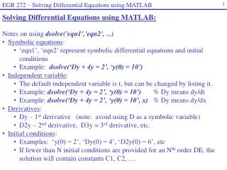
OPTIMIZATION SOFTWARE as a Tool for Solving Differential Equations Using NEURAL NETWORKS. Fotiadis, D. I. Karras, D. A. Lagaris, I. E. Likas, A. Papageorgiou, D. G. DIFFERENTIAL EQUATIONS HANDLED. ODE’s Systems of ODE’s PDE’s ( Boundary and Initial Value Problems )

E N D
OPTIMIZATION SOFTWAREas a Tool for Solving Differential Equations UsingNEURAL NETWORKS Fotiadis, D. I. Karras, D. A. Lagaris, I. E. Likas, A. Papageorgiou, D. G.
DIFFERENTIAL EQUATIONS HANDLED • ODE’s • Systems of ODE’s • PDE’s ( Boundary and Initial Value Problems ) • Eigen - Value PDE Problems • IDE’s
ARTIFICIAL NEURAL NETWORKS • Closed Analytic Form • Universal Approximators • Linear and Non-Linear Parameters • Highly Parallel Systems • Specialized Hardware for ANN
OPTIMIZATION ENVIRONMENT MERLIN / MCL 3.0 SOFTWARE • Features Include: • A Host of Optimization Algorithms • Special Merit for Sums of Squares • Variable Bounds and Variable Fixing • Command Driven User Interface • Numerical Estimation of Derivatives • Dynamic Programming of Strategies
Input Layer Hidden Layers Output Layer (1) w (2) w x 1 1 1 x 2 2 2 v Bias + 1 3 u ARTIFICIALNEURAL NETWORKS • Inspired from biological NN Input - Output mapping via the weightsu,w,v and the activation functionss Analytically this is given by the formula:
Activation Functions Many different functions can be used. Our current choice: The Sigmoidal A smooth function, infinitely differentiable, bounded in (0,1)
FACTS Kolmogorov and Cybenko and Hornik proved theorems concerning the approximation capabilities of ANNs In fact it is shown that ANNs are UNIVERSAL APPROXIMATORS
DESCRIPTION OF THE METHOD SOLVE THE EQUATION SUBJECT TO DIRICHLET B.C. Where Lis an Integrodifferential Operator Linear or Non-Linear
Where: • B(x)satisfies the BC • Z(x)vanishes on the boundary • N(x)is an Artificial Neural Net
MODEL PROPERTIES The Model satisfies by construction the B.C. The Model thanks to the Network is“trainable” The Network parameters can be adjusted so that:
Pick a set of representative points in the unit Hypercube The residual “Error”
ILLUSTRATION Simple 1-d example Model
ILLUSTRATION For a second order, two-dimensional PDE: where
EXAMPLES Problem: Solve the 2-d PDE: In the domain: Subject to the BC : A single hidden layer Perceptron was used:
GRAPHICAL REPRESENTATION The analytic solution is: Exact
GRAPHS & COMPARISON Neural Solution accuracy Plot Points: Training Points
GRAPHS & COMPARISON Neural Solution accuracy Plot Points: Test Points
GRAPHS & COMPARISON Finite Element Solution accuracy Plot Points: Training Points
GRAPHS & COMPARISON Finite Element Solution accuracy Plot Points: Test Points
PERFORMANCE • Highly Accurate Solution (even with few training points) • Uniform “Error” Distribution • Superior Interpolation Properties The model solution is very flexible. Can be easily enhanced to offer even higher accuracy.
Problem: With appropriate Dirichlet BC EIGEN VALUE PROBLEMS The model is the same as before. However the “Error” is defined as:
EIGEN VALUE PROBLEMS Where: i.e. the value for which the “Error” is minimum. Problems of that kind are often encountered in Quantum Mechanics. (Schrödinger’s equation)
EXAMPLES The non-local Schrödinger equation Describes the bound “n+a” system in the framework of the Resonating Group Method. Model: Where: is a single hidden layer, sigmoidal Perceptron
OBTAINING EIGENVALUES Example:The Henon-Heiles potential Asymptotic behavior: Model used: Use the above model to obtain an eigen solution F. Obtain a different eigen solution by deflation, i.e. : This model is orthogonal to F(x,y) by construction. The procedure can be applied repeatedly.
Let be the set of the training points inside the domain. ARBITRARILY SHAPED DOMAINS For domains other than Hypercubes the BC cannot be embedded in the model. be the set of points Let defining the arbitrarily shaped boundary. The BC are then: We describe two ways to proceed solving the problem
OPTIMIZATION WITH CONSTRAINTS Model: “Error” to be minimized: Domain terms+Boundary terms With b a penalty parameter, to control the degree of satisfaction of the BC.
PERCEPTRON-RBF SYNERGY Model: Where the a’s are determined in a way so that the model satisfies the BC exactly, i.e.: The free parameter l is chosen once initially so as the system above is easily solved. “Error”:
Pros&Cons. . . The RBF - Synergy is: • Computationally costly. A linear system is solved each time the model is evaluated. • Exact in satisfying the BC. The Penalty method is: • Approximate in satisfying the BC. • Computationally efficient
IN PRACTICE . . . • Initially proceed via the penalty method, till an approximate solution is found. • Refine the solution, using the RBF- Synergy method, to satisfy the BC exactly. Conclusions: Experiments on several model problems shows performance similar to the one reported earlier.
GENERALOBSERVATIONS • Enhancedgeneralization performance is achieved, when the exponential weights of the Neural Networks are kept small. • Hence box-constrainedoptimization methods should be applied. • BiggerNetworks (greater number of nodes) can achieve higheraccuracy. • This favorsthe use of: • Existing Specialized Hardware • Sophisticated Optimization Software
MERLIN 3.0 A software package offering many optimization algorithms and a friendly user interface. What is it ? What problems does it solve ? Find a local minimum of the function: Under the conditions:
ALGORITHMS Direct Methods • SIMPLEX • ROLL Gradient Methods Conjugate Gradient Quasi Newton • BFGS (3 versions) • DFP • Polak-Ribiere • Fletcher-Reeves • Generalized P&R Levenberg-Marquardt • For Sum-Of-Squares
THE USER’S PART What the user has to do ? • Program the objective function • Use Merlin to find an optimum What the user may want to do ? • Program the gradient • Program the Hessian • Program the Jacobian
MERLIN FEATURES & TOOLS • Intuitive free-format I/O • Menu assisted Input • On-line HELP • Several gradient modes • Confidence parameter intervals • Box constraints • Postscript graphs • Programmability • “Open” to user enhancements
Merlin Control Language MCL: What is it ? High-Level Programming Language, that Drives Merlin Intelligently. What are the benefits ? • Abolishes User Intervention. • Optimization Strategies. • Handy Utilities. • Global Optimum Seeking Methods.
MCL REPERTOIRE MCL command types: • Merlin Commands • Conditionals (IF-THEN-ELSE-ENDIF) • Loops(DO type of loops) • Branching(GO TO type) • I/O(READ/WRITE) MCL intrinsic variables: All Merlin important variables, e.g.: Parameters, Value, Gradient, Bounds ...
SAMPLE MCL PROGRAM program var i; sml; bfgs_calls; nfix; max_calls sml = 1.e-4 %Gradient threshlod. bfgs_calls = 1000 %Number of BFGS calls. max_calls = 10000 %Max. calls to spend. again: loosall nfix = 0 loop i from 1 todim ifabs[grad[i]] <= sml then fix (x.i) nfix = nfix+1 end if end loop if nfix ==dimthen display 'Gradient below threshold...' loosall finish end if bfgs (noc=bfgs_calls) whenpcount < max_calls just move toagain display 'We probably failed...' end
MERLIN-MCLAvailability The Merlin - MCL package is written in ANSI Fortran 77 and can be downloaded from the following URL: http://nrt.cs.uoi.gr/merlin/ It is maintained, supported and is FREELY available to the scientific community.
FUTURE DEVELOPMENTS • Optimal Training Point Sets • Optimal Network Architecture • Expansion & Pruning Techniques Hardware Implementation on NEUROPROCESSORS