Download
1 / 38
380 likes | 535 Views
Lecture 3 Benchmarks and Performance Metrics. Measurement Tools. Benchmarks, Traces, Mixes Cost, Delay, Area, Power Estimation Simulation (many levels) ISA, RT, Gate, Circuit Queuing Theory Rules of Thumb Fundamental Laws. Plane. Time (DC-Paris). Speed. Passengers.

E N D
Lecture 3Benchmarks and Performance Metrics CS510 Computer Architectures
Measurement Tools • Benchmarks, Traces, Mixes • Cost, Delay, Area, Power Estimation • Simulation (many levels) • ISA, RT, Gate, Circuit • Queuing Theory • Rules of Thumb • Fundamental Laws CS510 Computer Architectures
Plane Time (DC-Paris) Speed Passengers Throughput (pmph) Boeing 747 BAD/Sud Concorde 6.5 hours 610 mph 470 286,700 3.0 hours 132 178,200 1350 mph The Bottom Line: Performance (and Cost) • Time to run the task (ExTime) • Execution time, response time, latency • Tasks per day, hour, week, sec, ns ....(Performance) • Throughput, bandwidth CS510 Computer Architectures
ExTime(Y) Performance(X) n = = ExTime(X) Performance(Y) The Bottom Line: Performance (and Cost) “X is n times faster than Y” means: CS510 Computer Architectures
ExTime(Y) Performance(X) n = = 1 + ExTime(X) Performance(Y) 100 100 x (Performance(X) - Performance(Y)) n = Performance(Y) Performance Terminology “X is n% faster than Y” means: CS510 Computer Architectures
ExTime(Y) ExTime(X) 15 10 1.5 1.0 Performance (X) Performance (Y) = = = 100 (1.5 - 1.0) 1.0 n = n = 50% Example Example: Y takes 15 seconds to complete a task, X takes 10 seconds. What % faster is X? CS510 Computer Architectures
Programs to Evaluate Processor Performance • (Toy) Benchmarks • 10~100-line program • e.g.: sieve, puzzle, quicksort • Synthetic Benchmarks • Attempt to match average frequencies of real workloads • e.g., Whetstone, dhrystone • Kernels • Time critical excerpts of real programs • e.g., Livermore loops • Real programs • e.g., gcc, spice CS510 Computer Architectures
Benchmarking Games • Differing configurations used to run the same workload on two systems • Compiler wired to optimize the workload • Workload arbitrarily picked • Very small benchmarks used • Benchmarks manually translated to optimize performance CS510 Computer Architectures
Common Benchmarking Mistakes • Only average behavior represented in test workload • Ignoring monitoring overhead • Not ensuring same initial conditions • “Benchmark Engineering” • particular optimization • different compilers or preprocessors • runtime libraries CS510 Computer Architectures
SPEC: System Performance Evaluation Cooperative • First Round 1989 • 10 programs yielding a single number • Second Round 1992 • SpecInt92 (6 integer programs) and SpecFP92 (14 floating point programs) • VAX-11/780 • Third Round 1995 • Single flag setting for all programs; new set of programs “benchmarks useful for 3 years” • SPARCstation 10 Model 40 CS510 Computer Architectures
800 700 600 500 SPEC Perf 400 300 200 100 0 li gcc doduc spice fpppp nasa7 eqntott tomcatv epresso matrix300 Benchmark SPEC First Round • One program: 99% of time in single line of code • New front-end compiler could improve dramatically CS510 Computer Architectures
How to Summarize Performance • Arithmetic Mean(weighted arithmetic mean) • tracks execution time:S (Ti)/norS Wi*Ti • Harmonic Mean(weighted harmonic mean) of execution rates (e.g., MFLOPS) • tracks execution time:n/S1/Riorn/SWi/Ri • Normalized execution timeis handy for scaling performance • But do not take the arithmetic mean of normalized execution time, use thegeometric meanP(Ri)1/n, where Ri=1/Ti CS510 Computer Architectures
Computer A Computer B Computer C Comparing and Summarizing Performance P1(secs) 1 10 20 P2(secs) 1,000 100 20 Total time(secs) 1,001 110 40 For program P1, A is 10 times faster than B, For program P2, B is 10 times faster than A, and so on... The relative performance of computer is unclear with Total Execution Times CS510 Computer Architectures
1 n • n • Execution Timei • i=1 • n • n • 1 / Ratei i=1 Ratei = • (1 / Execcution Timei) Summary Measure Arithmetic Mean Harmonic Mean(When performance is expressed as rates) Good, if programs are run equally in the workload CS510 Computer Architectures
n • n • Execution Time Ratioi i=1 Normalized to the reference machine Unequal Job Mix Relative Performance • Weighted Execution Time • Weighted Arithmetic Mean • Weighted Harmonic Mean • n • Weighti x Execution Timei • i=1 • n • Weighti / Ratei i=1 • Normalized Execution Time to a reference machine • Arithmetic Mean • Geometric Mean CS510 Computer Architectures
W(i)j x Timej n WAM(i) = j=1 A B CW(1)W(2)W(3) P1 (secs) 1.00 10.00 20.00 0.50 0.909 0.999 P2(secs) 1,000.00 100.00 20.00 0.50 0.091 0.001 1.0 x 0.5 + 1,000 x 0.5 Weighted Arithmetic Mean WAM(1) 500.50 55.00 20.00 WAM(2) 91.91 18.19 20.00 WAM(3) 2.00 10.09 20.00 CS510 Computer Architectures
n A B C P1 1.00 10.00 20.00 P2 1,000.00 100.00 20.00 Geometric Mean = n • Execution time ratioi I=1 Normalized to A Normalized to B Normalized to C A B C A B C A B C Normalized Execution Time P1 1.0 10.0 20.0 0.1 1.0 2.0 0.05 0.5 1.0 P2 1.0 0.1 0.02 10.0 1.0 0.2 50.0 5.0 1.0 Arithmetic mean 1.0 5.05 10.01 5.05 1.0 1.1 25.03 2.75 1.0 Geometric mean 1.0 1.0 0.63 1.0 1.0 0.63 1.58 1.58 1.0 Total time 1.0 0.11 0.04 9.1 1.0 0.36 25.03 2.75 1.0 CS510 Computer Architectures
Normalized to A Normalized to B Normalized to C A B C A B C A B C P1 P2 Arithmetic mean B is 5 times slower than A A is 5 times slower than B C is slowest C is fastest Disadvantages of Arithmetic Mean Performance varies depending on the reference machine 1.0 10.0 20.0 0.1 1.0 2.0 0.05 0.5 1.0 1.0 0.1 0.02 10.0 1.0 0.2 50.0 5.0 1.0 1.0 5.05 10.01 5.05 1.0 1.1 25.03 2.75 1.0 CS510 Computer Architectures
Normalized to A Normalized to B Normalized to C A B C A B C A B C The Pros and Cons Of Geometric Means • Independent of running times of the individual programs • Independent of the reference machines • Do not predict execution time • the performance of A and B is the same : only true when P1 ran 100 times for every occurrence of P2 1(P1) x 100 + 1000(P2) x 1 = 10(P1) x 100 + 100(P2) x 1 P1 1.0 10.0 20.0 0.1 1.0 2.0 0.05 0.5 1.0 P2 1.0 0.1 0.02 10.0 1.0 0.2 50.0 5.0 1.0 Geometric mean 1.0 1.0 0.63 1.0 1.0 0.63 1.58 1.58 1.0 CS510 Computer Architectures
Speedup due to enhancement E: ExTime w/o E Performance w/E Speedup(E) = = ExTime w/ E Performance w/o E Amdahl's Law Suppose that enhancement E accelerates a fraction F of the task by a factor S, and the remainder of the task is unaffected, then: ExTime(E) = Speedup(E) = CS510 Computer Architectures
FractionE ExTimeE = ExTime x (1 - FractionE) + SpeedupE 1 ExTime ExTimeE Speedup= = (1 - FractionE) + FractionE SpeedupE 1 = (1 - F) + F/S Amdahl’s Law CS510 Computer Architectures
1 Speedup = (1-F) + F/S 1 1 = = = 1.053 (1-0.1) + 0.1/2 0.95 5.3% improvement Amdahl’s Law Floating point instructions are improved to run 2 times(100% improvement); but only 10% of actual instructions are FP CS510 Computer Architectures
Memory Disk / Tape Reg’s Cache Corollary(Amdahl):Make the Common Case Fast • All instructions require an instruction fetch, only a fraction require a data fetch/store • Optimize instruction access over data access • Programs exhibit locality Spatial Locality Temporal Locality • Access to small memories is faster • Provide a storage hierarchy such that the most frequent accesses are to the smallest (closest) memories. CS510 Computer Architectures
Locality of Access Spatial Locality: There is a high probability that a set of data, whose address differences are small, will be accessed in small time difference. Temporal Locality: There is a high probability that the recently referenced data will be referenced in near future. CS510 Computer Architectures
Rule of Thumb • The simple case is usually the most frequent and the easiest to optimize! • Do simple, fast things in hardware(faster) and be sure the rest can be handled correctly in software CS510 Computer Architectures
Application Answers per month Operations per second Programming Language Compiler (millions) of Instructions per second: MIPS (millions) of (FP) operations per second: MFLOP/s ISA Datapath Megabytes per second Control Function Units Cycles per second (clock rate) Transistors Wires Pins Metrics of Performance CS510 Computer Architectures
Seconds Instructions Cycles Seconds CPU time = = x x Program Program Instruction Cycle Inst Count CPI Clock Rate Aspects of CPU Performance Program X Compiler X (X) Inst. Set. X X Organization X Technology X X CS510 Computer Architectures
Normalized: • add,sub,compare, mult 1 • divide, sqrt 4 • exp, sin, . . . 8 • Normalized: • add,sub,compare, mult 1 • divide, sqrt 4 • exp, sin, . . . 8 Marketing Metrics • MIPS = Instruction Count / Time x 106 = Clock Rate / CPI x 106 • Machines with different instruction sets ? • Programs with different instruction mixes ? • Dynamic frequency of instructions • Not correlated with performance • MFLOP/s = FP Operations / Time x 106 • Machine dependent • Often not where time is spent CS510 Computer Architectures
n CPU time = Cycle Time x SCPI x I i i i = 1 n CPI = SCPI x F ,where F = I i i i i i = 1 Instruction Count Invest resources where time is spent ! Cycles Per Instruction Average cycles per instruction • CPI = (CPU Time x Clock Rate) / Instruction Count • = Cycles / Instruction Count Instruction Frequency CS510 Computer Architectures
Application Programming Language Compiler Datapath Control Function Units Transistors Wires Pins Organizational Trade-offs Instruction Mix CPI ISA Cycle Time CS510 Computer Architectures
Op Freq CPI(i) CPI (% Time) Typical Mix Example: Calculating CPI Base Machine (Reg / Reg) ALU 50% 1 .5 (33%) Load 20% 2 .4 (27%) Store 10% 2 .2 (13%) Branch 20% 2 .4 (27%) 1.5 CS510 Computer Architectures
Op Freqi CPIi ALU50%1 Load20%2 Store10%2 Branch20%2 Typical Mix Example Some of LD instructions can be eliminated by having R/M type ADD instruction [ADD R1, X] • Add register / memory operations: R/M • One source operand in memory • One source operand in register • Cycle count of 2 • Branch cycle count to increase to 3 • What fraction of the loads must be eliminated for this to pay off? Base Machine (Reg / Reg) CS510 Computer Architectures
Op Freqi CPIi CPI ALU .50 1.5 Load .202.4 Store .10 2.2 Branch .20 2.4 Total1.001.5 Example Solution Exec Time = Instr Cnt x CPI x Clock CS510 Computer Architectures
New Freqi CPIi CPINEW .5 - X 1.5 - X .2 - X 2.4 - 2X .1 2.2 .2 3.6 X 22X 1 - X(1.7 - X)/(1 - X) CPINEW must be normalized to new instruction frequency Example Solution Exec Time = Instr Cnt x CPI x Clock Old Op Freqi CPIi CPI ALU.50 1 .5 Load.202 .4 Store.10 2 .2 Branch.202 .4 Reg/Mem 1.00 1.5 CS510 Computer Architectures
Old New Op Freq Cycles CPIOld Freq Cycles CPINEW ALU.50 1 .5.5 - X1.5 - X Load.20 2 .4.2 - X2.4 - 2X Store.10 2 .2.12 .2 Branch.20 2 .4.23.6 Reg/MemX22X 1.00 1.51 - X(1.7 - X)/(1 - X) Instr CntOldx CPIOldx Clock = Instr CntNew x CPINewx Clock 1.00 x 1.5 = (1 - X) x (1.7 - X)/(1 - X) 1.5 = 1.7 - X 0.2 = X Example Solution Exec Time = Instr Cnt x CPI x Clock All LOADs must be eliminated for this to be a win ! CS510 Computer Architectures
Fallacies and Pitfalls • MIPS is an accurate measure for comparing performance among computers • dependent on the instruction set • varies between programs on the same computer • can vary inversely to performance • MFLOPS is a consistent and useful measure of performance • dependent on the machine and on the program • not applicable outside the floating-point performance • the set of floating-point operations is not consistent across the machines CS510 Computer Architectures