Download
1 / 30
310 likes | 471 Views
DSP architectures for wireless communications. Sridhar Rajagopal Department of Electrical and Computer Engineering Rice University, Houston TX ECE Pizza Talk March 28, 2003. This work has been supported in part by Nokia, TI, TATP and NSF. Wireless Cellular. Wireless LAN. Bluetooth/

E N D
DSP architectures for wireless communications Sridhar Rajagopal Department of Electrical and Computer Engineering Rice University, Houston TX ECE Pizza Talk March 28, 2003 This work has been supported in part by Nokia, TI, TATP and NSF
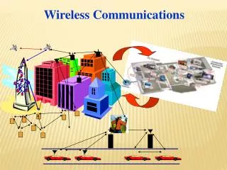
Wireless Cellular Wireless LAN Bluetooth/ Home Networks Future wireless devices : • High data rate mobile devices with multimedia • Multiple antennas w/ complex algorithms, GOPs of computation • Area-Time-Power constraints • Seamless connection across environments and standards • Use the fastest and cheapest available service
Design me Aim of the talk
Trends FLEXIBILITY
Application Layer Network Layer MAC Layer Physical Layer Change in flexibility requirements No change (already flexible) Maximum change (needs to support multiple environments, algorithms and standards)
Programmable Area-Time-Power benefits Intermediate Flexibility Time-to-market Software updates ASICs Architecture trade-offs Past : more DSP + less ASIC, Current : less DSP + more ASIC Reason: need less flexibilityOR DSPs not powerful enough? Can’t we build better DSPs? How much flexibility do we need?
Problems with current DSPs • Current DSPs • Not enough functional units (FUs) for GOPs of computation • Need 100’s of FUs • Not low power enough!! • Cannot extend to more FUs • Limited Instruction Level Parallelism (ILP) • Limited Subword Parallelism (such as MMX) • Cannot support more registers (area,ports) • Compilers: difficult to find ILP as FUs increase
Scalable Wireless Application-specific Procesors (SWAPs) • Exploit data parallelism (DP) • Available in many wireless algorithms • This is what ASICs do!! • Example: int i,a,b,c; // 32 bits short int d,e,f; // 16 bitspacked for (i = 1; i<= 1024; ++i) { a[i] = b[i] + c[i]; d[i] = e[i] + f[i]; } DP ILP Subword
Input Data Kernel Stream Output Data Interference Cancellation receivedsignal Matched filter Viterbi decoding Decoded bits Correlator channel estimation SWAPs: stream processors for wireless • Kernels (computation) and streams (communication) • Operations on kernels use local data • Streams expose data parallelism • Imagine stream processor at Stanford
+ + + + Internal Memory + + + + … ILP + + + + * * * * * * * * * * * * + + DP ILP + * * * DSP vs. SWAPs Stream Register File (SRF) SWAPs (max. clusters All clusters same & do same operations) DSP (1 cluster)
Arithmetic clusters From/To SRF Local Register File • FUs (+,*,/) • Scratch-pad (Sp) • Indexed accesses • Comm. unit (CU) • Intercluster comm. • Distributed reg. Files • more FUs + + + + + + * * + + * * SRF / Cross Point / / / Sp Intercluster Network CU
SWAPs vs. DSPs trade-offs • Same internal memory size as DSPs • Dependent on application, not architecture • Needs more area to support more functional units • Area is less of a constraint than power • Varying levels of DP in applications • Needs reconfiguration!! • Need to turn off unused clusters (and FUs) • More parallelism lower clock frequency lower voltage low power (CV2f + leakage) in spite of larger area
Design methodology Chain of receiver algorithms Low “complexity”, parallel, fixed point Flexibility- performance tradeoffs High level language implementation Architecture exploration FPGA, customized, reconfigurable, heterogeneous designs ASIC design learn learn Modular programmable architecture design DSP, SWAPs H-SWAPs
Baseband processing Antenna Detection Decoding Higher (MAC/Network/OS) Layers RF Front-end Channel estimation Physical layer of wireless receivers Receiver more complex than transmitter
Algorithms for • Multiple antenna systems (MIMO systems) • Complexity exponential with transmit * receive antennas • Wide range of extremely complex algorithms • Optimal depends on fading, mobility, bandwidth, antennas • GOPs of computations • Estimation: Linear MMSE, blind, conjugate gradient…. • Detection: FFT, (blind) interference cancellation…. • Decoding: Viterbi, Turbo, LDPC…. • Implement ALL of them AND the NEXT one in line • Use for the best for the situation Example for concept demonstration: Viterbi decoding
Parallel Viterbi Decoding • 1. Add-Compare-Select (ACS) : trellis interconnect • Parallelism depends on constraint length (#states) • 2. Conventional Traceback • Sequential (No DP) • Difficult to implement in parallel architecture • Use Register Exchange (RE) • parallel solution
b. Shuffled Trellis a. Trellis X(0) X(0) X(0) X(0) X(1) X(1) X(1) X(2) X(2) X(2) X(2) X(4) X(3) X(3) X(6) X(3) X(8) X(4) X(4) X(4) X(10) X(5) X(5) X(5) X(12) X(6) X(6) X(6) X(7) X(14) X(7) X(7) X(8) X(8) X(8) X(1) X(9) X(9) X(9) X(3) X(10) X(5) X(10) X(10) X(11) X(11) X(7) X(11) X(12) X(9) X(12) X(12) X(13) X(13) X(11) X(13) X(13) X(14) X(14) X(14) X(15) X(15) X(15) X(15) Re-ordering for parallel Viterbi Exploiting Viterbi DP in SWAPs: • Re-order ACS, RE • Overhead
SWAP: Algorithms + Architecture Algorithm design for parallelism Architecture design?
+ + + + … ? ? ? ? ILP * * * * * * * * DP SWAP design • Decide how many clusters • Exploit DP • Decide what to put within each cluster • Maximize ILP with high functional unit efficiency • Search design space with “explore” tool • See how it meets time-area-power constraints
(80,34) (85,24) (85,17) 160 (85,13) 140 (85,11) (70,59) 120 (73,41) 100 (62,62) Instruction count (76,33) 80 (72,22) (65,45) (54,59) (43,58) (72,19) (47,43) (61,33) 60 (39,41) (60,26) (49,33) 40 (61,22) (40,32) (48,26) 1 1 (39,27) (50,22) 2 2 (39,22) 3 3 #Multipliers #Adders 4 4 5 5 Inside a SWAP cluster: EXPLORE Auto-exploration of adders and multipliers for “ACS" (Adder FU%, Multiplier FU%)
“Explore” tool benefits • Instruction count vs. functional unit efficiency • What goes inside each cluster • Explore all algorithms • turn off functional units not in use for given kernel • Design customized application-specific units • Better performance with increased FU utilization Algorithm 1 : 3 adders, 3 multipliers, 32 clusters Algorithm 2 : 4 adders, 1 multiplier, 64 clusters Architecture: 4 adders, 3 multipliers, 64 clusters
Viterbi reconfiguration DP Can be turned OFF Packet 1 Constraint length 7 (16 clusters) Packet 2 Constraint length 9 (64 clusters) Packet 3 Constraint length 5 (4 clusters)
Viterbi decoding: rate 1/2 at 128 Kbps = 10 MHz 1000 K = 9 K = 7 Static architecture DSP K = 5 SWAPs 100 Frequency needed to attain real-time (in MHz) 10 1 1 10 100 Number of clusters Ideal C64x (w/o co-proc) needs ~200 MHz for real-time
SWAPs : Salient features • 1-2 orders of magnitude better than 1 processor DSP • Any constraint length 10 MHz at 128 Kbps • Same code for all constraint lengths • no need to re-compile or load another code • as long as parallelism/cluster ratio is constant • Power savings due to dynamic cluster scaling
Viterbi Clusters used Peak Power K = 9 64 ~90 mW K = 7 16 ~28.57 mW K = 5 4 ~13.8 mW overhead 0 ~8.1 mW 90 80 70 60 50 Power (in mW) 40 30 20 10 0 0 10 20 30 40 50 60 70 Active Clusters (max 64) Expected SWAP power consumption • 64 clusters and 1 multiplier per cluster: • 0.13 micron, 1.2 V • Peak Active Power: ~9 mW at 1 MHz • Area: ~53.7 mm2 • 10 MHz, 128 Kbps with reconfiguration *Exploring the VLSI Scalability of Stream Processors, Brucek Khailany et al, Proceedings of the Ninth Symposium on High Performance Computer Architecture, February 8-12, 2003, Anaheim, California, USA, pp. 153-164
Flexibility vs. performance • Suitable for mobile devices? • SWAPs: Real-time at ~10-100 mW • Maybe ; but can we do better? • ASICs : Real-time at ~10-100 W • No special customization for the application • No application-specific units • Generic inter-cluster communication network • Overhead for extracting parallelism • SWAPs suitable for base-stations? • Why not? – power is not a primary constraint!
100000 FAST MEDIUM DSP SLOW 10000 32-user base-station 1000 Frequency needed to attain real-time (in MHz) 100 Mobile 10 100 1 10 Number of clusters Multiuser Estimation-Detection+Decoding Real-time target : 128 Kbps per user Ideal C64x (w/o co-proc) needs ~15 GHz for real-time
Current research • SWAPs : Completely flexible and general • How do we trade-off flexibility for better performance? • Handset SWAPs (H-SWAPs)
DSP (RE) Partial DP + Task Pipelining Application-specific units DP SWAP H-SWAP Task Pipelining Dedicated interconnect Dedicated interconnect ASIC/FPGA – Real-time performance ASIC/FPGA – Real-time performance H-SWAPs: Potential advantages DSP (RE) Execution time SWAPs H-SWAPs
Conclusions • Need flexible architectures for future wireless devices • Higher data rates, lower power, more complex algorithms • Design methodology (SWAPs, H-SWAPs, ASICs) • Flexibility vs. performance trade-offs • Blurs distinction between ASICs and programmable solutions • Also need parallel, low precision algorithms for efficient mapping • Inter-disciplinary research: • Computer architecture, VLSI, wireless communications, computer arithmetic, compilers