From the text we are given -
330 likes | 353 Views
This text discusses various methods for estimating depths and resistivity in resistivity measurements, including the interpolation approach, inflection point estimation, extrapolation, and the method of characteristic curves.

From the text we are given -
E N D
Presentation Transcript
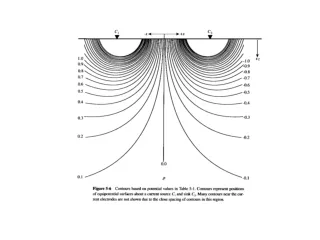
From the text we are given - z is depth and d is electrode spacing
In the preceding diagram z was depth. In this diagram z is depth divided by a which is 1/3rd the current electrode separation. Remember the a-spacing is referred to in the context of the Wenner Array.
Change in potential d in this case is the distance between the source electrode and nearby potential electrode; i.e a in the case of the Wenner array. Note the similarity of this “sensitivity” curve to the relative response function (V(z)) used with terrain conductivity data. You can also think of this curve as indicating the contribution of intervals at various depths to the potential between one current and one potential electrode.
We see that in general for the Wenner array the peak sensitivity of the array to subsurface resistivity distributions occurs at depths approximately equal to the a-spacing.
By comparison to the characterization of instrument response as a function of depth and intercoil spacing these relationships are defined much more qualitatively for the resistivity applications.
Qualitative interpretation of a resistivity sounding - How many layers have been sensed in this resistivity sounding? The observations consist of apparent resistivities recorded at various a-spacings (Wenner array) or l-spacings (Schlumberger array).
Let’s examine the utility of the interpolation approach using synthetic data. Synthetic data are data that have been calculated from a model. Thus we know what the actual answer should be. Refer to your handout. Given the potential how do we determine apparent resistivity?
The apparent resistivities (a) are computed from the relationship we derived earlier. WhereG= 2a for the Wenner array
Here are some plots of our synthetic or “test” data set. The model from which it is derived is shown at lower right.
The Inflection Point Depth Estimation Procedure This technique suggests that the depths to various boundaries are related to inflection points in the apparent resistivity measurements. Again, the In-Class data set illustrates the utility of this approach. Apparent resistivities plotted below are shown over the model for both the Schlumberger and Wenner arrays. The inflection points are located, and dropped to the spacing-axis. The technique is suggested too be most applicable for use with the Schlumberger array. The inflection point rule varies with array type. For the Wenner array, the approximate depth to the interface is 1/2 the inflection point spacing. For the Schlumberger array this would give a depth to the top of the layer of about 12 meters instead of the actual depth of 8. In the case of the Wenner array we would get a depth of about 9 meters. A general “rule of thumb” for the Schlumberger array would to divide the inflection point distance by 3 instead of 2; that would yield 8 meters.
Resistivity determination through extrapolation This technique suggests that the actual resistivity of a layer can be estimated by extrapolating the trend of apparent resistivity variations toward some asymptote, as shown in the figure below. The problem with this is being able to correctly guess where the plateau or asymptote actually is. Spacings in the In-Class data set only go out to 50 meters. The model data set (below) used for the inflection point discussion reveals that this asymptote is reached only gradually, in this case at distances of 500 meters and greater. Since most of the layers affecting the apparent resistivity in our surveys will be associated with thin layers, we are unlikely to be able to do this very accurately. The apparent resistivity will vary considerably over that distance rather than rise gradually to resistivities of individual layers. At best the technique offers only a crude estimate.
Method of Characteristic curves The curves are calculated responses for given conditions. The curves shown at right are for a two-layer model. We’ll consider this method in more detail during lecture next Thursday.
Frohlich used the method of characteristic curves to estimate the depths to resistivity interfaces and their resistivity. We’ll talk more about the method of characteristic curves in the next lecture.