Download
1 / 45
450 likes | 466 Views
This paper introduces a batch mode active learning approach for large-scale text categorization, aiming to minimize human labeling effort while building efficient classifiers. The approach utilizes convex optimization formulation and eigen space simplification to find informative examples for labeling. Experimental results demonstrate the effectiveness of the proposed method.

E N D
Large-Scale TextCategorization ByBatch Mode Active Learning Steven C.H. Hoi†, Rong Jin‡, Michael R. Lyu† † CSE Department, Chinese University of Hong Kong ‡ CSE Department, Michigan State University 26-May, 2006 To appear in International World Wide Web conference, Edinburgh, Scotland, 22-26 May, 2006.
Outline • Introduction • Related Work • Batch Mode Active Learning • Theoretical Foundation • Convex Optimization Formulation • Eigen Space Simplification • Bound Optimization Algorithm • Experimental Results • Conclusion and Future Work
Introduction • Text Categorization • Problem • Assign documents to predefined topics • Significances • Core Web data mining technique • Applications: category browsing, vertical search, etc. • Challenges • To build efficient classifiers • To minimize human labeling effort
Introduction • Logistic Regression • Efficiency for Training and Prediction • Natural Probability Output • State-of-the-art performance, etc… • Linear model where is the class label. Simplified notation:
Introduction • Active Learning • To find most informative unlabeled examples • Traditional Methodology • Choose one unlabeled example for labeling • Retrain the classifier with the additional example • Limitation • Only one example in each iteration, huge retraining cost • Our solution: Batch Mode Active Learning • To find a batch of most informative unlabeled examples
Outline • Introduction • Related Work • Batch Mode Active Learning • Theoretical Foundation • Convex Optimization Formulation • Eigen Space Simplification • Bound Optimization Algorithm • Experimental Results • Conclusion and Future Work
Related Work • Statistical Models for Classification • K Nearest Neighbors (Masand et al., SIGIR’92), Decision Trees (Apte et al., TOIS’94), Bayesian Classifiers (Tzeras et al., SIGIR’93), Inductive Rule Learning (Cohen et al., ICML’95), etc. • Neural Networks (Ruiz et al., IR’02), Support Vector Machines (SVM) (Joachims, ECML’98, Tong et al., ICML’00), and Logistic Regressions (Zhang et al., ICML’00), etc.
Related Work • Active Learning • Query-By-Committee (Liere et al AAAI’97), EM & Active Learning (Nigam et al’98), etc. • Margin Based Methods: Support Vector Machine Active Learning (Tong et al., ICML’00) • Measure uncertainty by the distances from decision boundaries
Batch Mode Active Learning • Toy Example – Positive examples of class-1 – Negative examples of class-2 – Unlabeled examples – Selected examples for labeling D1 D2 (a) Binary classification example (b) Margin-based active learning (c) Batch mode active learning
Outline • Introduction • Related Work • Batch Mode Active Learning • Theoretical Foundation • Convex Optimization Formulation • Eigen Space Simplification • Bound Optimization Algorithm • Experimental Results • Conclusion and Future Work
Theoretical Foundation • Main Idea: • Based on the theoretical framework of maximization of Fisher information • Problem Setting In a probabilistic classification framework, assume the classification model is a semi-parametric form For example, the logistic regression model:
Theoretical Foundation • The problem of batch mode active learning can be regarded as a problem to seek a resample distribution q(x) of the unlabeled data. • The examples with large resampling probabilities will be selected as the most informative ones for labeling. • According to statistical estimation theory, active learning should consider a resample distribution q(x) that maximizes the following Fisher information
Theoretical Foundation • The maximization of Fisher information is equivalent to find the resample distribution q(x) that minimizes the ratio of two Fisher information matrixes: • For the logistic regression model, the Fisher information matrix can be expressed as: • We replace the integration in the above equation with the summation over the unlabeled data:
Convex Optimization Formulation • Rewrite the objective function as • Introduce a slack matrix ,then turn the original problem into the following optimization: • In the above, we use
Convex Optimization Formulation • By the Schur complementary theorem, i.e., • we turn it into the following optimization :
Convex Optimization Formulation • The final optimization problem can be expressed • The above problem belongs to the family of Semi-definite programming (SDP) and can be solved by convex optimization techniques.
Eigen Space Simplification • Directly solving the above optimization problem is computationally expensive for the large-size slack matrix variable of M. • In order to reduce the computational complexity, we propose an Eigen space simplification method to make the solution simpler and more effective. • We assume that Mis expanded in the Eigen space of the Fisher information matrix Ip.
Eigen Space Simplification • Let be the top seigen vectors of the Fisher information matrix Ip, where λ1≥ λ2≥ . . . ≥ λs, then we assume the matrix Mhas the following form: • We rewrite the inequality
Eigen Space Simplification • Using the eigen expression, we have • Given the necessary condition for is • Therefore, we have the following result
Eigen Space Simplification • The above necessary condition leads to following constraints: • Meanwhile, the objective function of tr(M) can be expressed as
Eigen Space Simplification • By putting the above two expressions together, we transform the SDP problem into the following approximate optimization problem: • Note that the above optimization problem belongs to convex optimization since f(x) = 1/xis convex when x ≥ 0.
Bound Optimization Algorithm • Lemma 1: Let L(q) be the objective function, we have the following conclusion:
Bound Optimization Algorithm • Given the lemma 1, now instead of optimizing the original objective function L(q), we can optimize its upper bound using simple updating equations:, • This algorithm will guarantee to converge to a local optimal. Since the original problem is a convex optimization problem, the above updating procedure will guarantee to converge to a global optimal.
Bound Optimization Algorithm • The updating step: • Some Observations • (i) The example with a large classification uncertaintywill be assigned with a large probability. • (ii) The example that is similar to many unlabeled examples is more likely to be selected.
Outline • Introduction • Related Work • Batch Mode Active Learning • Theoretical Foundation • Convex Optimization Formulation • Eigen Space Simplification • Bound Optimization Algorithm • Experimental Results • Conclusion and Future Work
Experimental Testbeds • 3 standard text datasets • Reuters-21578 dataset (10788) • Two web-related datasets: WebKB (4518) and Newsgroup (10966)
Experimental Settings • A standard feature selection by Information Gain is conducted to remove uninformative features, in which 500 of the most informative features are selected. • The F1 metric is adopted as our evaluation metric, which has been shown to be more reliable metric than other metrics such as the classification accuracy. More specifically, the F1 is defined as where p and r are precision and recall. • Parameters of LogReg and SVM are determined by a standard cross validation method.
Comparison Schemes • Two popular active learning methods: • SVM-AL: the classification uncertainty of an example x is determined by its distance to the decision boundary The smaller the distance d(x;w, b) is, the more the classification uncertainty will be. • LogReg-AL: the logistic regression active learning algorithm that measures the classification uncertainty based on the entropy of the distribution p(y|x). The larger the entropy of x is, the more uncertain we are about the class labels of x. • Our Batch Mode Active Learning algorithm with logistic regression, i.e., LogReg-BMAL in short.
Empirical Evaluation • Experimental Results with Reuters-21578 • average results over 40 executions • 100 training examples and 100 active examples
Empirical Evaluation • Experimental Results with Reuters-21578
Empirical Evaluation • Experimental Results with Reuters-21578
Empirical Evaluation • Experimental Results with Web-KB Dataset
Empirical Evaluation • Experimental Results with Newsgroup Dataset
Conclusion • A batch mode active learning scheme is proposed to attack the challenge of large-scale text categorization. • The main contributions include • A new active learning scheme is suggested for large-scale text categorization to overcome the limitation of traditional active learning; • A batch mode active learning solution is formulated by convex optimization techniques; • An effective bound optimization algorithm is proposed to solve the batch mode active learning problem • Extensive experiments are conducted for empirical evaluations in comparisons with state-of-the-art active learning approaches for text categorization
Future Work • To combine batch mode active learning with semi-supervised learning • To improve the computational costs • To study the convergence of the bound optimization • To extend the methodology for other classification models
Thank you for your attention! Questions? Http://www.cse.cuhk.edu.hk/~chhoi/
Appendix A – Statistical Estimation Theory • Given a semi-parametric model, say the logistic model as: • In theory, one can use the maximum-likelihood estimate (MLE) to determine the model parameter as: • In theory, the MLE achieves the Cramer-Rao lower bound, thus, the MLE is the asymptotically most efficient estimator, whose efficiency can be measured by the Fisher information that is intrinsic to the probability model.
Appendix A – Statistical Estimation Theory (cont.) • More specifically, the expected log-likelihood to measure the goodness of q(x) can be given as • Hence, according to the Crammer-Rao lower bound, the MLE based on the resample distribution q(x) that minimizes is the most efficient estimator of alpha among all estimators based on a resampling of x. • Therefore, the result of q to solve the optimization is the optimal sample distribution for active learning.
Appendix B. Fisher Information and Cramer-Rao lower bound • Fisher information is thought of as the amount of information that an observable random variable X carries about an unobservable parameter θ upon which the probability distribution of X depends. Since the expectation of the score is zero, the variance is also the second moment of the score and so the Fisher information can be written • In statistics, the Cramér-Rao lower bounds express a lower bound on the accuracy of a statistical estimator, based on Fisher information. • It states that the reciprocal of the Fisher information, , of a parameter θ, is a lower bound on the variance of an unbiased estimator of the parameter (denoted ).
Appendix C – Convexity Theorem Theorem. Any locally optimal point of a convex problem is (globally) optimal.
Appendix E: Proof of Lemma1 • Lemma 1: Let L(q) be the objective function in (15), we have the following conclusion • Proof.
Proof (cont.):Using the convexity property of reciprocal function, namely for x ≥ 0 and p.d.f. . We can arrive the following deduction
Proof (cont.):Substituting the above inequation back to L(q), we can attain the following inequality: This finishes the proof of the inequality lemma. □