Download
1 / 80
860 likes | 1.11k Views
10. PARAMETRIC EQUATIONS AND POLAR COORDINATES. PARAMETRIC EQUATIONS & POLAR COORDINATES. So far, we have described plane curves by giving: y as a function of x [ y = f ( x )] or x as a function of y [ x = g ( y )]

E N D
10 PARAMETRIC EQUATIONS AND POLAR COORDINATES
PARAMETRIC EQUATIONS & POLAR COORDINATES • So far, we have described plane curves by giving: • y as a function of x [y = f(x)] or x as a function of y [x = g(y)] • A relation between x and y that defines y implicitly as a function of x [f(x, y) = 0]
PARAMETRIC EQUATIONS & POLAR COORDINATES • In this chapter, we discuss two new methods for describing curves.
PARAMETRIC EQUATIONS • Some curves—such as the cycloid—are best handled when both x and y are given in terms of a third variable t called a parameter [x = f(t), y = g(t)].
POLAR COORDINATES • Other curves—such as the cardioid—have their most convenient description when we use a new coordinate system, called the polar coordinate system.
PARAMETRIC EQUATIONS & POLAR COORDINATES 10.1Curves Defined by Parametric Equations • In this section, we will learn about: • Parametric equations and generating their curves.
INTRODUCTION • Imagine that a particle moves along the curve C shown here. • It is impossible to describe C by an equation of the form y = f(x). • This is because C fails the Vertical Line Test.
INTRODUCTION • However, the x- and y-coordinates of the particle are functions of time. • So, we can write x = f(t) and y = g(t).
INTRODUCTION • Such a pair of equations is often a convenient way of describing a curve and gives rise to the following definition.
PARAMETRIC EQUATIONS • Suppose x and y are both given as functions of a third variable t (called a parameter) by the equations x = f(t) and y = g(t) • These are called parametric equations.
PARAMETRIC CURVE • Each value of t determines a point (x, y),which we can plot in a coordinate plane. • As t varies, the point (x, y) = (f(t), g(t)) varies and traces out a curve C. • This is called a parametric curve.
PARAMETER t • The parameter t does not necessarily represent time. • In fact, we could use a letter other than t for the parameter.
PARAMETER t • However, in many applications of parametric curves, t does denote time. • Thus, we can interpret (x, y) = (f(t), g(t)) as the position of a particle at time t.
PARAMETRIC CURVES Example 1 • Sketch and identify the curve defined by the parametric equations x = t2 – 2ty = t + 1
PARAMETRIC CURVES Example 1 • Each value of t gives a point on the curve, as in the table. • For instance, if t = 0, then x = 0, y = 1. • So, the corresponding point is (0, 1).
PARAMETRIC CURVES Example 1 • Now, we plot the points (x, y) determined by several values of the parameter, and join them to produce a curve.
PARAMETRIC CURVES Example 1 • A particle whose position is given by the parametric equations moves along the curve in the direction of the arrows as t increases.
PARAMETRIC CURVES Example 1 • Notice that the consecutive points marked on the curve appear at equal time intervals, but not at equal distances. • That is because the particle slows down and then speeds up as t increases.
PARAMETRIC CURVES Example 1 • It appears that the curve traced out by the particle may be a parabola. • We can confirm this by eliminating the parameter t, as follows.
PARAMETRIC CURVES Example 1 • We obtain t = y– 1 from the equation y = t + 1. • We then substitute it in the equation x = t2– 2t. • This gives: x = t2 – 2t = (y – 1)2 – 2(y – 1) = y2 – 4y + 3 • So, the curve represented by the given parametric equations is the parabola x = y2 – 4y + 3
PARAMETRIC CURVES • This equation in x and y describes where the particle has been. • However, it doesn’t tell us when the particle was at a particular point.
ADVANTAGES • The parametric equations have an advantage––they tell us when the particle was at a point. • They also indicate the direction of the motion.
PARAMETRIC CURVES • No restriction was placed on the parameter t in Example 1. • So, we assumed t could be any real number. • Sometimes, however, we restrict t to lie in a finite interval.
PARAMETRIC CURVES • For instance, the parametric curve • x = t2 – 2ty = t + 1 0 ≤ t ≤4 • shown is a part of the parabola in Example 1. • It starts at the point (0, 1) and ends at the point (8, 5).
PARAMETRIC CURVES • The arrowhead indicates the direction in which the curve is traced as t increases from 0 to 4.
INITIAL & TERMINAL POINTS • In general, the curve with parametric equations • x = f(t) y = g(t) a≤ t ≤ b • has initial point (f(a), g(a)) and terminal point (f(b), g(b)).
PARAMETRIC CURVES Example 2 • What curve is represented by the following parametric equations? • x = cos t y = sin t 0 ≤ t ≤ 2π
PARAMETRIC CURVES Example 2 • If we plot points, it appears the curve is a circle. • We can confirm this by eliminating t.
PARAMETRIC CURVES Example 2 • Observe that: • x2 + y2 = cos2 t + sin2 t = 1 • Thus, the point (x, y) moves on the unit circle x2 + y2 = 1
PARAMETRIC CURVES Example 2 • Notice that, in this example, the parameter t can be interpreted as the angle (in radians), as shown.
PARAMETRIC CURVES Example 2 • As t increases from 0 to 2π, the point (x, y) = (cos t, sin t) moves once around the circle in the counterclockwise direction starting from the point (1, 0).
PARAMETRIC CURVES Example 3 • What curve is represented by the given parametric equations? • x = sin 2ty = cos 2t 0 ≤ t ≤ 2π
PARAMETRIC CURVES Example 3 • Again, we have: • x2 + y2 = sin2 2t + cos2 2t = 1 • So, the parametric equations again represent the unit circle x2 + y2 = 1
PARAMETRIC CURVES Example 3 • However, as t increases from 0 to 2π, the point (x, y) = (sin 2t, cos 2t) starts at (0, 1), moving twicearound the circle in the clockwise direction.
PARAMETRIC CURVES • Examples 2 and 3 show that different sets of parametric equations can represent the same curve. • So, we distinguish between: • A curve, which is a set of points • A parametric curve, where the points are traced in a particular way
PARAMETRIC CURVES Example 4 • Find parametric equations for the circle with center (h, k) and radius r.
PARAMETRIC CURVES Example 4 • We take the equations of the unit circle in Example 2 and multiply the expressions for x and y by r. • We get: x = r cos ty = r sin t • You can verify these equations represent a circle with radius r and center the origin traced counterclockwise.
PARAMETRIC CURVES Example 4 • Now, we shift h units in the x-direction and k units in the y-direction.
PARAMETRIC CURVES Example 4 • Thus, we obtain the parametric equations of the circle with center (h, k) and radius r : • x = h + r cos t y = k + r sin t 0 ≤ t ≤ 2π
PARAMETRIC CURVES Example 5 • Sketch the curve with parametric equations x = sin ty = sin2 t
PARAMETRIC CURVES Example 5 • Observe that y = (sin t)2 = x2. • Thus, the point (x, y) moves on the parabola y = x2.
PARAMETRIC CURVES Example 5 • However, note also that, as -1 ≤ sin t ≤ 1, we have -1 ≤ x ≤ 1. • So, the parametric equations represent only the part of the parabola for which -1 ≤ x ≤ 1.
PARAMETRIC CURVES Example 5 • Since sin t is periodic, the point (x, y) = (sin t, sin2 t) moves back and forth infinitely often along the parabola from (-1, 1) to (1, 1).
GRAPHING DEVICES • Most graphing calculators and computer graphing programs can be used to graph curves defined by parametric equations. • In fact, it’s instructive to watch a parametric curve being drawn by a graphing calculator. • The points are plotted in order as the corresponding parameter values increase.
GRAPHING DEVICES Example 6 • Use a graphing device to graph the curve x = y4 – 3y2 • If we let the parameter be t = y, we have the equations x = t4 – 3t2y = t
GRAPHING DEVICES Example 6 • Using those parametric equations, we obtain this curve.
GRAPHING DEVICES Example 6 • It would be possible to solve the given equation for y as four functions of x and graph them individually. • However, the parametric equations provide a much easier method.
GRAPHING DEVICES • In general, if we need to graph an equation of the form x = g(y), we can use the parametric equations x = g(t) y = t
GRAPHING DEVICES • Notice also that curves with equations y = f(x) (the ones we are most familiar with—graphs of functions) can also be regarded as curves with parametric equations x = ty = f(t)
GRAPHING DEVICES • Graphing devices are particularly useful when sketching complicated curves.