Download
1 / 6
60 likes | 191 Views
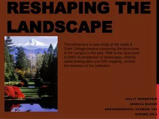
Reshaping the Landscape. The following is a case study of the Lewis & Clark College campus comparing the land cover of the campus in the year 1936 to the land cover of 2005. A comparison of landscapes, utilizing aerial photographs and GIS mapping, unfolds the evolution of the institution. .

E N D
Reshaping the Landscape The following is a case study of the Lewis & Clark College campus comparing the land cover of the campus in the year 1936 to the land cover of 2005. A comparison of landscapes, utilizing aerial photographs and GIS mapping, unfolds the evolution of the institution. Sally Bernstein Jessica Kleiss Environmental Studies 330 Spring 2012
GEOREFERENCED AERIAL PHOTOS Campus 2005 Campus 1936 I chose to compare 1936 and 2005 because I wanted to look at the oldest aerial photo to the newest. I used 2005 as the present because it was the most recent photo available (although there is a 2006 photography, for unknown reasons GIS would not process it). I decided to use 1936 because I wanted to look at how campus has evolved from its ‘original’ landscape to that of present day. I chose to georeference ‘landmark’ points on campus—those being the reflecting pool, the frank manor house, the gatehouse, and so forth. Due to unknown error, only a handful of GPS points were processed into GIS. Unfortunately those that were successfully processed fell in an almost perfect line making it more difficult to obtain a variety of distributions.
Land Cover Change Campus 2005 Campus 1936 I chose the following three variables to explore. Impervious Surfaces included the entirety of the built environment (roads, sidewalks, athletic fields/courts, pools, and buildings). Grass covers all areas of well-kept lawns and gardens (all maintained ‘natural’ areas). Forest includes all unmaintained areas consisting of mainly trees. I wanted to keep grass and forest separate because I wanted to look at how the untouched (and mainly forested) areas of the 1936 campus evolved to satisfy the community demand (both physical needs and aesthetics).
Quantitative Analysis 1936 1936 Total Acreage: 82.962 In 1936, 3% of campus was impervious 2005 2005 Total Acreage: 92.48 In 2005, 50% of the campus was impervious
Discussion • My analysis showed a significant increase in impervious surfaces between the chosen years 1936 and 2005. In 1936 only 3% of the campus was covered in impervious surfaces, compared to 2005 where 50% of the campus was impervious. This illustrates an enormous increase. However, the extreme jump in impervious surfaces gives reason for the decline in forest and grass. Interestingly, impervious surface was the only variable with such an extreme and significant disparity. Forest and grass account for 82% of the 1936 campus, and 48% of the 2005 campus. Although this is a large decrease, the campus still remains almost half covered in permeable surfaces. • The increase impervious surface is not surprising due to the large growth in the institutions population and academic needs. As the institution has grown, the growing community has created a need and demand for the addition of pathways, expansion and creation of parking lots, and the construction of new academic and residential facilities. These all account for the significant increase of impermeable surface areas. Although buildings, parking lots, and synthetic athletic fields (the football field) have been constructed, the school continues to emphasize ‘green’ and ‘environmental’ values. This could reason for why the expansions have not eradicated ‘natural areas’—and why forest and grass remains covering almost half of the undergraduate campus. • The creation and expansion of impermeable surfaces come with a greater potential for negative environmental impacts. The construction of these spaces and places disrupts native habitats, transforms the geography of the land, and introduces greater human presence within the given space (from forest to the academic core). All these constructions pose a risk for run-off, reduction of natural vegetation and native species, increasing emissions, and eradication of natural habitats.
Errors & Bias • This analysis had a great potential for error. Human error could have heavily weighed in on the construction of the GIS maps. Free-form drawing polygons over the aerial photographs can account for one element of human error. On a similar note, the photographs were not crystal clear, the blur and uncertainty of area type (grass, forest, and impermeable) could have again caused for a second degree of human error. Lastly, human error could have occurred in the collection and georeferencing of waypoints. Since georeferencing relied on personal perception and decisions of where the point was taken, verses where the point found itself on the photographs, the plotting of GPS points on aerial photographs may have been skewed. In my analysis not all of the GPS points were able to process, this caused all points to fall along the same trajectory. A wider distribution of waypoints would have created a more accurate map (in line with the campus boundary). For example on my georeferenced maps, the flag pole matches perfectly with the 1936 photograph, but imperfectly with the 2005 photograph. If there had been more waypoints included, with a greater spread, the photo may have georeferenced more accurately. • Calculation errors weighed into the analysis particularly when calculating statistical analysis. The total area of the campus boundary in 1936 was ~82 acres. The total area of the campus in 2005 increased by 10 acres, creating a total coverage of ~92 acres. This disparity in total acreage may have skewed both perception and calculations of polygon areas. • Having completed an almost identical project the past fall (fall 2011), I had a notion of what the map should look like. This could have created a bias, because I knew what my map should look like. Additionally, my familiarity with the campus could have created a bias as well.