Download
1 / 19
280 likes | 646 Views
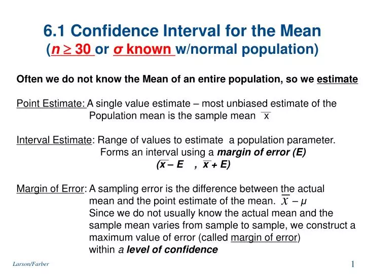
6.1 Confidence Interval for the Mean ( n 30 or σ known w/normal population ). Often we do not know the Mean of an entire population, so we estimate Point Estimate: A single value estimate – most unbiased estimate of the Population mean is the sample mean x

E N D
6.1 Confidence Interval for the Mean(n 30 or σknown w/normal population) Often we do not know the Mean of an entire population, so we estimate Point Estimate: A single value estimate – most unbiased estimate of the Population mean is the sample mean x Interval Estimate: Range of values to estimate a population parameter. Forms an interval using a margin of error (E) (x – E , x + E) Margin of Error: A sampling error is the difference between the actual mean and the point estimate of the mean. – μ Since we do not usually know the actual mean and the sample mean varies from sample to sample, we construct a maximum value of error (called margin of error) within a level of confidence Larson/Farber
Point estimate 12.4 • Estimating the Population Mean μ Market researchers use the number of sentences per advertisement as a measure of readability for magazine advertisements. The following represents a random sample of the number of sentences found in 50 advertisements. Find a point estimate of the population mean, . (Journal of Advertising Research) 9 20 18 16 9 9 11 13 22 16 5 18 6 6 5 12 25 17 23 7 10 9 10 10 5 11 18 18 9 9 17 13 11 7 14 6 11 12 11 6 12 14 11 9 18 12 12 17 11 20 Your point estimate for the mean length of all magazine advertisements is 12.4 sentences. Interval estimate : An interval, or range of values, used to estimate a population parameter. How confident do we want to bethat the interval estimate contains the population mean μ? (90%, 95%, 80%??? - This determines what our margin of error will be. 10.3 14.5 ( ) Interval estimate (with margin of error = 2.1) Larson/Farber
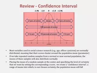
c ½(1 – c) ½(1 – c) z -zc z = 0 zc Confidence Intervals c is the area under the standard normal curve between the critical values. Level of confidence c • The probability that the interval estimate contains the population parameter. Use the Standard Normal Table to find the corresponding z-scores. Critical values • If the level of confidence is 90% (c = .90) this means that we are 90% confident that the interval contains the population mean μ. • There is 10% left for the ‘tails’ of the distribution. (5% for each tail = .05) • -zc = invnorm (.05) = -1.645 and zc = invnorm (.95) = 1.645 Larson/Farber 4th ed
0.95 0.025 0.025 z z = 0 zc Margin of Error (E) • Greatest possible distance between the point estimate and the value of the parameter it is estimating for a given level of confidence, c. • Sometimes called the maximum error of estimate or error tolerance. Example:Use the magazine advertisement data and a 95% confidence level to find the margin of error for the mean number of sentences in all magazine advertisements. Assume the sample standard deviation (s) is about 5.0. 95% of the area under the curve falls within 1.96 standard deviations of the mean. Ti 83/84 Stat-Tests 7:Zinterval () When n 30, the sample standard deviation, s, can be used for . -zc= -1.96 zc= 1.96 11.0 < μ < 13.8 E= 1.96 (5/√50) = 1.4 sentences. A 95% confidence interval for the population mean (Probability confidence interval contains μ is 95%) (x – E , x + E) (12.4 – 1.4 , 12.4 + 1.4) = (11 , 13.8) Larson/Farber
Constructing Confidence Intervals for μ Finding a Confidence Interval for a Population Mean (n 30 or σknown with a normally distributed population) In Words In Symbols • Find the sample statistics n and • Specify , if known. Otherwise, if n 30, find the sample standard deviation s and use it as an estimate for . • Find the critical value zc that corresponds to the given level of confidence. • Find the margin of error E. • Find the left and right endpoints and form the confidence interval. Std. Norm. Table -> InvNorm() Interval: Interpretation: “If a large number of samples is collected and a confidence interval is created for each sample, approximately C% of these intervals will contain μ.” Larson/Farber
Practice A publisher wants to estimate the mean length of time (in minutes) All adults spend reading newspapers. To determine this estimate, the publisher takes a random sample of 15 people and obtains the following results. 11, 9, 8, 10, 10, 9, 7, 11, 11, 7, 6, 9, 10, 8, 10 From past studies, the publisher assumes a population std deviation of 1.5 minutes And that the population is Normally Distributed Construct a 90% and 99% confidence interval for the population mean. Larson/Farber
0.95 0.025 0.025 z z = 0 zc Sample Size Given a c-confidence level & a margin of error E, the minimum sample size n needed to estimate the population mean is (If is unknown you can estimate it with ‘s’ if sample >= 30) Example: You want to estimate the mean number of sentences in a magazine advertisement. How many magazine advertisements must be included in the sample if you want to be 95% confident that the sample mean is within one sentence of the population mean? Assume the sample std. deviation is about 5.0. -zc= -1.96 zc= 1.96 You should include at least 97 magazine advertisements in your sample Larson/Farber
d.f. = 2 d.f. = 5 6.2 Confidence Interval for Mean (σ unknown) • When the population standard deviation is unknown, the sample size is less than 30, and the random variable x is approximately normally distributed, it follows a t-distribution(critical values are denoted tc) w/properties below: The t-distribution is bell shaped and symmetric about the mean. The t-distribution is a family of curves, each determined by a parameter called the degrees of freedom. When estimating a population mean, the degrees of freedom= n – 1 • The total area under a t-curve is 1 or 100%. • The mean, median, and mode of the t-distribution are equal to zero. • As the degrees of freedom increase, t-distribution approaches the normal distribution. After 30 d.f., t-distribution is very close to the standard normal z-distribution. The tails in the t-distribution are “thicker” than those in the standard normal distribution. 0 t Standard normal curve Larson/Farber
c = 0.95 t -tc = -2.145 tc =2.145 Example: Critical Values of t Solution: d.f. = n – 1 = 15 – 1 = 14 95% of the area under the t-distribution curve with 14 degrees of freedom lies between t = +2.145. Find the critical value tc for a 95% confidence when the sample size is 15. tc = 2.145 A c-confidence interval for the population mean μ (The probability that the confidence interval contains μis c. Larson/Farber
Confidence Intervals and t-Distributions In Words In Symbols • Identify the sample statistics n, , and s. • Identify the degrees of freedom, level of confidence c, and the critical value tc. • Find the margin of error E. • Find the left and right endpoints & find the confidence interval. d.f. = n – 1 Larson/Farber
Example: Constructing a Confidence Interval You randomly select 16 coffee shops and measure the temperature of the coffee sold at each. The sample mean temperature is 162.0ºF with a sample standard deviation of 10.0ºF. Find the 95% confidence interval for the mean temperature. Assume the temperatures are approximately normally distributed. Use t-distribution (n < 30, σ unknown, approximate normal distribution) • n =16, x = 162.0 s = 10.0 c = 0.95 • df = n – 1 = 16 – 1 = 15 • tc = 2.131 Margin of Error Confidence Interval (162 – 5.3, 162 +5.3) = (156.7, 167.3) 156.7 < μ < 167.3 With 95% confidence, you can say that the mean temperature of coffee sold is between 156.7ºF and 167.3ºF. Ti 83/84 Stat-Tests 8:Tinterval () Larson/Farber
z-Normal Distribution OR t-Distribution? z t Note: You must have reason to believe you are working with an approximately normal distribution to use the t-distribution. If n 30, then according to the Central Limit Theorem the sampling distribution of the sample means approximates a normal distribution, so you have met this part of the criteria. Additionally, if n 30, the t-distribution is very close to the standard normal z-distribution so actually you could use either the z or t distribution, though your book guides you to use a “t” in this situation since the standard deviation of the population is unknown. If n < 30 and the population is not normally distributed (or you do not know) then you cannot use the standard normal (z) or the t-distribution. .
Example: Normal(z) or t-Distribution? You randomly select 25 newly constructed houses. The sample mean construction cost is $181,000 and the population standard deviation is $28,000. Assuming construction costs are normally distributed, should you use the normal distribution, the t-distribution, or neither to construct a 95% confidence interval for the population mean construction cost? Solution: Use the normal (z) distribution (the population is normally distributed and the population standard deviation is known) Larson/Farber
Practice Assume the variable is normally distributed and use (as appropriate) a normal distribution or t-distribution to construct a 90% confidence interval for the population mean. A) In a random sample of 10 adults from the U.S., the mean waste generated Per person per day was 4.54 pounds and the standard deviation was 1.21 pounds. B) Repeat part (a), assuming the same statistics came from a sample size of 500. Note that the sample size is quite large (much greater than 30). Construct a 90% confidence interval for the population mean first using a z-standard normal distribution, then again using a t-distribution. Compare The two answers and consider the reason for your results. Larson/Farber
6.3 Confidence Interval for Population Proportions Recall that ‘p’ is the probability of success in a binomial experiment. Just as we estimated the mean, we can estimate population proportions (p). Point Estimate for p (“p-hat”) Point Estimate for q (“q-hat”) A binomial distribution can be approximated by the normal distribution. If np >= 5 and nq >=5 is approximately ‘normal’. A c-confidence interval for the population proportion p (The probability that the confidence interval contains p is c.) Example: A survey of 1219 U.S. adults: 354 said that their favorite sport to watch is football. Find a point estimate for the population proportion of U.S. adults who say their favorite sport to watch is football. (The Harris Poll)
Constructing Confidence Intervals for p In Words In Symbols • Identify the sample statistics n and x. • Find the point estimate • Verify that the sampling distribution of can be approximated by the normal distribution. • Find the critical value zc that corresponds to the given level of confidence c. • Find the margin of error, E. • Find left & right endpoints and find confidence interval. Use Standard Normal Table Larson/Farber
Example: Confidence Interval for p In a survey of 1219 U.S. adults, 354 said that their favorite sport to watch is football. Construct a 95% confidence interval for the proportion of adults in the United States who say that their favorite sport to watch is football. Solution: Recall • Verify the sampling distribution of can be approximated by the normal distribution Ti 83/84 Stat-Tests A:1-PropZInt • Margin of error: invNorm (.975) = 1.96 0.265 < p < 0.315 + E • Confidence Interval: - E to With 95% confidence, you can say that the proportion of adults who say football is their favorite sport is between 26.5% and 31.5%. Larson/Farber
Sample Size • Given a c-confidence level and a margin of error E, the minimum sample size n needed to estimate p is • This formula assumes you have an estimate for and . • If not, use and Example: You are running a political campaign and wish to estimate, with 95% confidence, the proportion of registered voters who will vote for your candidate. Your estimate must be accurate within 3% of the true population. Find the minimum sample size needed if 1) no preliminary estimate is available and 2) a preliminary estimate gives = .31 #1: Since you do not have a preliminary estimate, use: Answer: 1068 voters #2: Use preliminary estimate: Answer: 914 voters Larson/Farber
Practice • You are a travel agent and wish to estimate with 95% confidence, the • Proportion of vacationers who plan to travel outside the U.S. in the next • 12 months. Your estimate must be accurate within 3% of the true proportion. • No preliminary estimate is available. Find the minimum sample size. • Find the minimum sample size needed, using a prior study that found that • 26% of the respondents said they planned to travel outside the • U.S. in the next 12 months. Larson/Farber