Download
1 / 52
540 likes | 655 Views
Foundations of Computer Vision. Lectures 09 Roger S. Gaborski. Exam 1 – Raw Scores. Exam 1- Percentage Scores. Assignment. How do you calculate the determinant of a 3 x 3 matrix? What are eigenvalues and how are they calculated? What are eigenvectors and how are they calculated?.

E N D
Foundationsof Computer Vision Lectures 09 Roger S. Gaborski
Assignment • How do you calculate the determinant of a 3 x 3 matrix? • What are eigenvalues and how are they calculated? • What are eigenvectors and how are they calculated?
Features • Match corresponding feature points in images • In video, two temporally adjacent frames • In still images, two different images of the same scene • Or two different images of similar scene
Issues • Lighting variations • View point • Scale • Rotation
NEED TO FIND CORRESPONDENCE BETWEEN FEATURE POINTS IN TWO DIFFERENT IMAGES • Cannot match individual pixels • Need to use a window containing many pixels (5x5, 7x7, 21x21, etc)
Matching on a continuum like texture and edges not very robust • Many edges (and parts of edges) will match • At the very least: • Need to find interest points • Extract patches around interest points • Match patches
Feature Points / Correspondence • Points should be extracted consistently over different views • Points should be invariant to scaling, rotation, changes in illumination • Information in the neighborhood of the point should be unique so that it can be matched
Select Window RegionMatch Region in Second Image Calculate difference between the two patches WindowMatching_ACV.m
Randomly Select Patch patch = I(80:110,200:230); For Demonstration Use Only Strip Containing Patch
This simple approach works because the patch was extracted from the image • We need a method that will work with ‘similar’ patches
Normalized Cross Correlation (Refer to equation on page p313)Also MATLAB docs • w is template • w is average value of elements in template • f is the image • f is the average of the image where f and w overlap • Denominator normalizes resulting in an output range of -1, +1 • High value for absolute value of output is a good match
MATLAB Cross Correlation Function g = normxcorr2(template, f)
Find Max Value in |g| d = abs(g); [ypeak, xpeak] = find(d == max(d(:))); %Adjust location by size of template %since g is larger than original image %by size of template ypeak = ypeak-(size(patch,1)-1)/2; xpeak = xpeak-(size(patch,2)-1)/2; fprintf('\n Center of Patch: ypeak is %d and xpeak is %d \n\n\n', ypeak, xpeak); figure, imshow(Igray) hold on plot(xpeak, ypeak, 'ro')
Red – strongest response Green – second strongest response (wheel rotation slightly different)
One Possible Approach • Read in Purple Flower Image and Select a 31x31 patch • Extract image strip that contains patch • Calculate Error=Absolute Difference Between Patch and Strip and plot • Repeat using Normalized Cross Correlation on whole image • Plot max location on image • CONTINUED NEXT SLIDE
One Possible Approach, continued • Repeat Normalized Cross Correlation using several different templates – choose templates from uniform areas and compare with templates containing strong edges, try different size templates • What are the characteristics of ‘good’ templates
Selection of Patches • We don’t want to just randomly select patches from an image • We want to select patches that have high information content • We want to do this automatically, not manually chosen
But How Do We Select Points? • Junctions or Corners • Stable over changes in viewpoint
Subtract First Window from Second Window Sightly Offset from First
Moravec’s Corner Detector • Overview: • Select window size • Shift window over image region • If window over uniform region, shifts in all directions will result in small changes • If window over edge, shifts along edge will results in small changes, but shifts across edge will result in large changes • along edge – no change • Perpendicular to edge – large change • If window over corner, than shifts in all directions will result will result in large changes • Detect corner by finding regions that have large changes in all directions
Subtract First Window from Second Window Window moved vertically, no change Window moved horizontally, no change Window moved in either direction, large change
Corner Detection: Basic Idea We should easily recognize the point by looking through a small window Shifting a window in anydirection should give a large change in intensity “flat” region:no change in all directions “edge”:no change along the edge direction “corner”:significant change in all directions Roger S. Gaborski Source: A. Efros
Wikipedia: Corner Detection-No shortage of corner detectors • Moravec • Harris • Laplacian of gaussians, Difference of Gaussian and Determinant of the Hessian • SIFT • SUSAN Corner Detector • Trajkovic – Hedley Corner Detector Roger S. Gaborski
Interest Point Detection • http://www.youtube.com/watch?v=_qgKQGsuKeQ
Corner Detection: Weighted Sum of Differences Window function Shifted intensity Intensity Window function w(u,v) = Area of patch: (u,v) or 1 in window, 0 outside Gaussian Change in appearance for the shift [x,y]: E(x,y) = ΣΣ w(u,v) (I(u+x, v+y) – I(u,v))2 u v Roger S. Gaborski Source: Wikipedia
Corner Detection: Mathematics Change in appearance for the shift [x,y]: I(u,v) E(x,y) E(3,2) E(0,0) Roger S. Gaborski Source: R. Szeliski
Corner Detection Change in appearance for the shift [x,y]: • E(x,y) = ΣΣ w(u,v) (I(u+x, v+y) – I(u,v))2 We want to find out how this function behaves for small shifts Roger S. Gaborski
Taylor Expansion Change in appearance for the shift [x,y]: • E(x,y) = ΣΣ w(u,v) (I(u+x, v+y) – I(u,v))2 Taylor expansion of I(u+x, v+y)= I(u,v) + Ix(u,v)*x + Iy(u,v)*y Ix and Iy are partial derivatives of x and y So, (I(u,v) + Ix(u,v)*x + Iy(u,v)*y – I(u,v))2 Results in E(x,y) = ΣΣ w(u,v) (Ix(u,v)*x+Iy(u,v)*y)2 Roger S. Gaborski
Corner Detection: Mathematics The approximation simplifies to E(x,y) = (x,y) A (x,y)T Where Ais a second moment matrixcomputed from image derivatives: A = ΣΣ w(u,v) Ix2IxIy IxIy Iy2 Roger S. Gaborski
Interpreting the second moment matrix Analyze eigenvalues of A to determine if a corner exists If λ1and λ2= 0, then pixel (x,y) is not of interest If one eigenvalue λ is close to 0, and the other is large, (x,y) is on an edge If both eigenvalues λ are large, (x,y) is a corner Roger S. Gaborski
Interpreting the eigenvalues Classification of image points using eigenvalues of M: 2 “Edge”2 >> 1 “Corner”1 and 2 are large,1 ~ 2;E increases in all directions 1 and 2 are small;E is almost constant in all directions “Edge”1 >> 2 “Flat” region 1 Roger S. Gaborski
Defining Corner Response Function, R Instead of calculating eigenvalues, Harris defined the following function: R = det(A)- α trace(A)2 = λ1λ2 - α (λ1 + λ2) Where α = .04 to .06 Recall: A = [ a b; c d] Det(A) = ad – bc Roger S. Gaborski
Corner Response Function R < 0 R > 0 Edge Corners |R| small R < 0 “Flat” region Edge Roger S. Gaborski
Harris Detector Algorithm • Compute Derivatives at each point • Compute Second Moment Matrix A • Compute Corner Response Function • Threshold R • Find Local Maxima Roger S. Gaborski
Harris Corner Detector • Reference: C.G. Harris and M.J. Stephens “A Combined Corner and Edge Detector” • Code inspired by Peter Kovesi • Derivative Masks: dx = [-1, 0, 1;-1, 0, 1;-1, 0, 1] • dy = dx’ • Image Derivatives; • Ix = imfilter(im, dx, 'conv',‘same’); • Iy = imfilter(im, dy, 'conv',‘same’); • Gaussian Filter • g = fspecial(‘gaussian’, 6*sigma, sigma); Roger S. Gaborski
Smooth squared image derivative • Ix2 = imfilter (Ix.^2, g, 'conv', ‘same’); • Iy2 = imfilter (Iy.^2, g, 'conv', ‘same’); • IxIy = imfilter (Ix .* Iy, g, 'conv', ‘same’); c = (Ix2.*Iy2 – IxIy.^2)./(Ix2+Iy2); Roger S. Gaborski
Non-maximal Suppression and Threshold • Extract local maxima – gray scale morphological dilation • size = 2*radius+1; %radius is parameter • mx = imdilate(c,ones(size)); %gray scale dilate • cc = (c==mx)&(c>thresh); %find maxima • [r,c] = find(cc) %find row, col coordinates • figure, imagesc( im), colormap(gray) • hold on • plot(c,r, ‘rs’), title(‘Corners) Roger S. Gaborski
100x100 Grid background =0, lines = 1 Roger S. Gaborski
Image rotated 45 Degrees Roger S. Gaborski
Image rotated 45 Degreessame parameters Roger S. Gaborski
Porsche Image Roger S. Gaborski