Download
1 / 10
100 likes | 166 Views
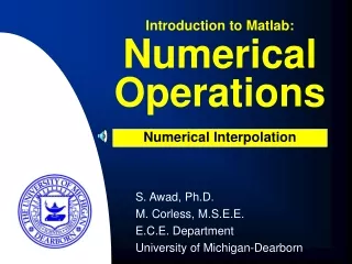
Introduction to Matlab:. Numerical Operations. Polynomial Manipulations. S. Awad, Ph.D. M. Corless, M.S.E.E. E.C.E. Department University of Michigan-Dearborn. Polynomial Topics. Entering Polynomials Roots Multiplication Evaluation Curve Fitting. Entering Polynomials.

E N D
Introduction to Matlab: Numerical Operations Polynomial Manipulations S. Awad, Ph.D. M. Corless, M.S.E.E. E.C.E. Department University of Michigan-Dearborn
Polynomial Topics • Entering Polynomials • Roots • Multiplication • Evaluation • Curve Fitting
Entering Polynomials • In Matlab, a polynomial is represented by a row vector of it’s coefficients in descending order • For example, the polynomial • Is entered as: » p=[1 -12 0 25 116] • Zero term coefficientsMUSTbe included
Roots • To find the roots of a polynomial use roots • Roots are always column vectors » p=[1 -12 0 25 116]; » r=roots(p) r = 11.7473 2.7028 -1.2251 + 1.4672i -1.2251 - 1.4672i
Mutliplication • Use the conv (convolution) command to evaluate the product of two polynomials: » a=[1 2 3 4];b=[1 4 9 16]; » c=conv(a,b) c = 1 6 20 50 75 84 64
Evaluation • polyval is used to evaluate the polynomial p(x) between -1 and 3 » x=linspace(-1,3); % 100 data points » p=[1 4 -7 -10]; % Coefficients » v=polyval(p,x); % Evaluate » plot(x,v); » title('x^3 +4x^2 -7x -10'); » xlabel('x');
Curve Fitting • polyfit implements a least squares curve fitting algorithm » x=[0:0.1:1]; » y=[-0.447 1.978 3.28 6.16 7.08 7.34 7.66 9.56 9.48 9.30 11.2]; » n=2; % Order of Fit » p=polyfit(x,y,n)
Polyfit • Polyfit returns coefficients of curve fit solution » p = polyfit(x,y,n) p = -9.8108 20.1293 -0.0317
Compare Solutions » xi=linspace(0,1,100); » z=polyval(p,xi); » plot(x,y,'-o',xi,z,':'); » xlabel('x'); » ylabel('y=f(x)'); » title('Second Order Curve Fitting'); • Least Mean Squared (LMS) Error Minimization