Test of Goodness of Fit

1. Test of Goodness of Fit Lecture 43 Section 14.1 – 14.3 Fri, Apr 8, 2005

2. Count Data • Count data – Data that counts the number of observations that fall into each of several categories. • The data may be univariate or bivariate. • Bivariate example – Observe a student’s final grade and class: A – F and freshman – senior.

3. Univariate Example • Observe students’ final grade in statistics: A, B, C, D, or F.

4. Bivariate Example • Observe students’ final grade in statistics and year in college.

5. Observed and Expected Counts • Observed counts – The counts that were actually observed in the sample. • Expected counts – The counts that would be expected if the null hypothesis were true. • In this chapter, we will entertain various null hypotheses.

6. The Chi-Square Statistic • Denote the observed counts by O and the expected counts by E. • Define the chi-square (2) statistic to be • Clearly, if the observed counts are close to the expected counts, then 2 will be small. • If even a few observed counts are far from the expected counts, then 2 will be large.

7. Think About It • Think About It, p. 853.

8. Chi-Square Degrees of Freedom • The chi-square distribution has an associated degrees of freedom, just like the t distribution. • Each chi-square distribution has a slightly different shape, depending on the number of degrees of freedom.

9. 2(2) 2(5) 2(10) Chi-Square Degrees of Freedom

10. Properties of 2 • The chi-square distribution with n degrees of freedom has the following properties. • 2  0. • It is unimodal. • It is skewed right. • 2 = n. • 2 = (2n). • If n is large, then 2(n) is approximately N(n, (2n)).

11. N(30,60) 2(30) N(32, 8) 2(32) Chi-Square vs. Normal

12. Chi-Square vs. Normal N(128, 16) 2(128)

13. The Chi-Square Table • See page 949. • The left column is degrees of freedom: 1, 2, 3, …, 15, 16, 18, 20, 24, 30, 40, 60, 120. • The column headings represent upper tails: • 0.005, 0.01, 0.025, 0.05, 0.10, • 0.90, 0.95, 0.975, 0.99, 0.995. • Of course, the upper tails 0.90, 0.95, 0.975, 0.99, 0.995 are the same as the lower tails 0.10, 0.05, 0.025, 0.01, 0.005.

14. Example • If df = 10, what value of 2 cuts off an upper tail of 0.05? • If df = 10, what value of 2 cuts off a lower tail of 0.05?

15. TI-83 – Chi-Square Probabilities • To find a chi-square probability on the TI-83, • Press DISTR. • Select 2cdf (item #7). • Press ENTER. • Enter the lower endpoint, the upper endpoint, and the degrees of freedom. • Press ENTER. • The probability appears.

16. Example • If df = 32, what is the probability that 2 will fall between 24 and 40? • Compute 2cdf(24, 40, 32). • If df = 128, what is the probability that 2 will fall between 96 and 160? • Compute 2cdf(96, 160, 128). • On the other hand, if df = 8, what is the probability that 2 will fall between 4 and 12? • Compute 2cdf(96, 160, 128).

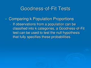
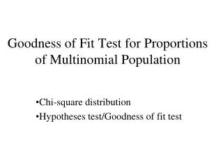
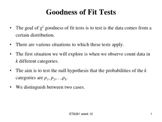
17. Tests of Goodness of Fit • The goodness-of-fit test applies only to univariate data. • The null hypothesis specifies a discrete distribution for the population. • We want to determine whether a sample from that population supports this hypothesis.

18. Examples • If we rolled a die 60 times, we expect 10 of each number. • If we got frequencies 8, 10, 14, 12, 9, 7, does that indicate that the die is not fair? • If we toss a fair coin, we should get two heads ¼ of the time, two tails ¼ of the time, and one of each ½ of the time. • Suppose we toss a coin 100 times and get two heads 16 times, two tails 36 times, and one of each 48 times. Is the coin fair?

19. Examples • If we selected 20 people from a group that was 60% male and 40% female, we would expect to get 12 males and 8 females. • If we got 15 males and 5 females, would that indicate that our selection procedure was not random (i.e., discriminatory)?

20. Null Hypothesis • The null hypothesis specifies the probability (or proportion) for each category. • Each probability is the probability that a random observation would fall into that category.

21. Null Hypothesis • To test a die for fairness, the null hypothesis would be H0: p1 = 1/6, p2 = 1/6, …, p6 = 1/6. • The alternative hypothesis would be H1: At least one of the probabilities is not 1/6.

22. Expected Counts • To find the expected counts, we apply the hypothetical probabilities to the sample size. • For example, if the hypothetical probability is 1/6 and the sample size is 60, then the expected count is (1/6)  60 = 10.

23. Example • We will use the sample data given for 60 rolls of a die to calculate the 2 statistic. • Make a chart showing both the observed and expected counts (in parentheses).

24. Example • Now calculate 2.

25. Computing the p-value • The number of degrees of freedom is 1 less than the number of categories in the table. • In this example, df = 5. • To find the p-value, use the TI-83 to calculate the probability that 2(5) would be at least as large as 3.4. • 2cdf(3.4, E99, 5) = 0.6386. • Therefore, p-value = 0.6386 (accept H0).

26. TI-83 – Goodness of Fit Test • The TI-83 will not automatically do a goodness-of-fit test. • The following procedure will compute 2. • Enter the observed counts into list L1. • Enter the expected counts into list L2. • Evaluate the expression (L1 – L2)2/L2. • Select LIST > MATH > sum and apply the sum function to the previous result. • The result is the value of 2.

27. Example • To test whether the coin is fair, the null hypothesis would be H0: pHH = 1/4, pTT = 1/4, pHT = 1/2. • The alternative hypothesis would be H1: At least one of the probabilities is not what H0 says it is.

28. Expected Counts • To find the expected counts, we apply the hypothetical probabilities to the sample size. • Expected HH = (1/4) 100 = 25. • Expected TT = (1/4)  100 = 25. • Expected HT = (1/2)  100 = 50.

29. Example • We will use the sample data given for 60 rolls of a die to calculate the 2 statistic. • Make a chart showing both the observed and expected counts (in parentheses).

30. Example • Now calculate 2.

31. Computing the p-value • In this example, df = 2. • To find the p-value, use the TI-83 to calculate the probability that 2(2) would be at least as large as 8.16. • 2cdf(8.16, E99, 2) = 0.0169. • Therefore, p-value = 0.0169 (reject H0).