Download

1 / 38
380 likes | 464 Views
Lecture 7 Overview. Two Key Network-Layer Functions. forwarding : move packets from router’s input to appropriate router output routing : determine route taken by packets from source to dest. routing algorithms Analogy routing : process of planning trip from source to destination

E N D
Two Key Network-Layer Functions • forwarding: move packets from router’s input to appropriate router output • routing: determine route taken by packets from source to dest. • routing algorithms • Analogy • routing: process of planning trip from source to destination • forwarding: process of getting through single interchange CPE 401/601 Lecture 7 : Routing
routing and forwarding routing algorithm local forwarding table header value output link 0100 0101 0111 1001 3 2 2 1 value in arriving packet’s header 1 0111 2 3 CPE 401/601 Lecture 7 : Routing
Connection setup • 3rd important function in some architectures • ATM, frame relay, X.25 • before datagrams flow, two end hosts and intervening routers establish virtual connection • routers get involved • network vs transport layer connection service: • network: between two hosts • may also involve intervening routers in case of VCs • transport: between two processes CPE 401/601 Lecture 7 : Routing
Network layer service models Guarantees ? Network Architecture Internet ATM ATM ATM ATM Service Model best effort BR VBR ABR UBR Congestion feedback no (inferred via loss) no congestion no congestion yes no Bandwidth none constant rate guaranteed rate guaranteed minimum none Loss no yes yes no no Order no yes yes yes yes Timing no yes yes no no CPE 401/601 Lecture 7 : Routing
Virtual Circuit Implementation • A Virtual Circuit consists of • path from source to destination • VC numbers • one number for each link along path • entries in forwarding tables in routers along path • Each packet carries VC identifier • VC number can be changed on each link • Every router on source-dest path maintains “state” for each passing connection CPE 401/601 Lecture 7 : Routing
Incoming interface Incoming VC # Outgoing interface Outgoing VC # 1 12 3 22 2 63 1 18 3 7 2 17 1 97 3 87 … … … … Forwarding table VC number 22 32 12 3 1 2 interface number Forwarding table in northwest router: Routers maintain connection state information! CPE 401/601 Lecture 7 : Routing
application transport network data link physical application transport network data link physical Virtual circuits: signaling protocols • used to setup, maintain teardown VC • used in ATM, frame-relay, X.25 • not used in today’s Internet 6. Receive data 5. Data flow begins 4. Call connected 3. Accept call 1. Initiate call 2. incoming call CPE 401/601 Lecture 7 : Routing
application transport network data link physical application transport network data link physical Datagram networks • no call setup at network layer • routers: no state about end-to-end connections • no network-level concept of “connection” • packets forwarded using destination host address • packets between same src-dst pair may take different paths 1. Send data 2. Receive data CPE 401/601 Lecture 7 : Routing
Forwarding table 4 billion possible entries Destination Address RangeLink Interface 11001000 00010111 00010000 00000000 through 0 11001000 00010111 00010111 11111111 11001000 00010111 00011000 00000000 through 1 11001000 00010111 00011000 11111111 11001000 00010111 00011001 00000000 through 2 11001000 00010111 00011111 11111111 otherwise 3 CPE 401/601 Lecture 7 : Routing
Longest prefix matching Prefix MatchLink Interface 11001000 00010111 00010 0 11001000 00010111 00011000 1 11001000 00010111 00011 2 otherwise 3 Examples Interface 0 DA: 11001000 00010111 00010110 10100001 DA: 11001000 00010111 00011000 10101010 Interface 1 Network Layer
Datagram or VC network: why? • Internet (datagram) • data exchange among computers • “elastic” service, no strict timing requirement • “smart” end systems (computers) • can adapt, perform control, error recovery • simple inside network, complexity at “edge” • many link types • different characteristics • uniform service difficult CPE 401/601 Lecture 7 : Routing
Datagram or VC network: why? • ATM (VC) • evolved from telephony • human conversation: • strict timing, reliability requirements • need for guaranteed service • “dumb” end systems • telephones • complexity inside network CPE 401/601 Lecture 7 : Routing
Lecture 8Routing Algorithms CPE 401 / 601 Computer Network Systems slides are modified from Dave Hollinger slides are modified from J. Kurose & K. Ross
5 3 5 2 2 1 3 1 2 1 x z w u y v Graph abstraction Graph: G = (N,E) N = set of routers = { u, v, w, x, y, z } E = set of links ={ (u,v), (u,x), (v,x), (v,w), (x,w), (x,y), (w,y), (w,z), (y,z) } Graph abstraction is useful in other network contexts Example: P2P, where N is set of peers and E is set of TCP connections CPE 401/601 Lecture 8 : Routing Algorithms
5 3 5 2 2 1 3 1 2 1 x z w u y v Graph abstraction: costs • c(x,x’) = cost of link (x,x’) • - e.g., c(w,z) = 5 • cost could always be 1, or inversely related to bandwidth, or inversely related to congestion Cost of path (x1, x2, x3,…, xp) = c(x1,x2) + c(x2,x3) + … + c(xp-1,xp) Question: What’s the least-cost path between u and z ? Routing algorithm: algorithm that finds least-cost path CPE 401/601 Lecture 8 : Routing Algorithms
Routing Algorithm classification • Global or decentralized information? • Global: link state algorithms • all routers have complete topology, • link cost info • Decentralized: distance vector algorithms • router knows physically-connected neighbors • link costs to neighbors • iterative process of computation, • exchange of info with neighbors CPE 401/601 Lecture 8 : Routing Algorithms
Routing Algorithm classification • Static or dynamic? • Static: • routes change slowly over time • Dynamic: • routes change more quickly • periodic update • in response to link cost changes CPE 401/601 Lecture 8 : Routing Algorithms
Dijkstra’s algorithm • A Link-State Routing Algorithm • Topology, link costs known to all nodes • accomplished via “link state broadcast” • all nodes have same info • Compute least cost paths from source node to all other nodes • produces forwarding table for that node • Iterative: • after k iterations, know least cost path to k dests CPE 401/601 Lecture 8 : Routing Algorithms
Dijkstra’s Algorithm Notation: • c(x,y): link cost from node x to y; • ∞ if not direct neighbors • D(v): current value of cost of path from source to dest v • p(v): predecessor node along path from source to v • N': set of nodes whose least cost path definitively known CPE 401/601 Lecture 8 : Routing Algorithms
Dijsktra’s Algorithm 1 Initialization: 2 N' = {u} 3 for all nodes v 4 if v adjacent to u 5 then D(v) = c(u,v) 6 else D(v) = ∞ 7 8 Loop 9 find w not in N' such that D(w) is a minimum 10 add w to N' 11 update D(v) for all v adjacent to w and not in N' : 12 D(v) = min( D(v), D(w) + c(w,v) ) 13 /* new cost to v is either old cost to v or known 14 shortest path cost to w plus cost from w to v */ 15 until all nodes in N‘ CPE 401/601 Lecture 8 : Routing Algorithms
5 3 5 2 2 1 3 1 2 1 x z w u y v Dijkstra’s algorithm: example D(v),p(v) 2,u 2,u 2,u D(x),p(x) 1,u D(w),p(w) 5,u 4,x 3,y 3,y D(y),p(y) ∞ 2,x Step 0 1 2 3 4 5 N' u ux uxy uxyv uxyvw uxyvwz D(z),p(z) ∞ ∞ 4,y 4,y 4,y CPE 401/601 Lecture 8 : Routing Algorithms
x z w u y v destination link (u,v) v (u,x) x y (u,x) (u,x) w z (u,x) Dijkstra’s algorithm: example Resulting shortest-path tree from u: Resulting forwarding table in u: CPE 401/601 Lecture 8 : Routing Algorithms
Dijkstra’s algorithm, discussion • Algorithm complexity: • n nodes • each iteration: need to check all nodes, w, not in N • n(n+1)/2 comparisons: O(n2) • more efficient implementations possible: O(nlogn) CPE 401/601 Lecture 8 : Routing Algorithms
D D C C A A A C D D A C B B B B Dijkstra’s algorithm, discussion • Oscillations possible: • e.g., link cost = amount of carried traffic 1 1+e 2+e 0 2+e 0 2+e 0 0 0 1 1+e 0 0 1 1+e e 0 0 0 e 1 1+e 0 1 1 e … recompute … recompute routing … recompute initially CPE 401/601 Lecture 8 : Routing Algorithms
Distance Vector Algorithm Bellman-Ford Equation • dynamic programming Define • dx(y) := cost of least-cost path from x to y Then • dx (y) = minv {c(x,v) + dv(y) } • where min is taken over all neighbors v of x CPE 401/601 Lecture 8 : Routing Algorithms
5 3 5 2 2 1 3 1 2 1 x z w u y v Bellman-Ford example Clearly, dv(z) = 5, dx(z) = 3, dw(z) = 3 B-F equation says: du(z) = min { c(u,v) + dv(z), c(u,x) + dx(z), c(u,w) + dw(z) } = min {2 + 5, 1 + 3, 5 + 3} = 4 Node that achieves minimum is next hop in shortest path ➜ forwarding table CPE 401/601 Lecture 8 : Routing Algorithms
Distance Vector Algorithm • Dx (y) = estimate of least cost from x to y • Node x knows cost to each neighbor v: c(x,v) • Node x maintains distance vector • Dx = [Dx (y): y є N ] • Node x also maintains its neighbors’ distance vectors • For each neighbor v, x maintains Dv = [Dv(y): y є N ] CPE 401/601 Lecture 8 : Routing Algorithms
Distance vector algorithm • Basic idea: • From time-to-time, each node sends its own distance vector estimate to neighbors • Asynchronous • When a node x receives new DV estimate from neighbor, it updates its own DV using B-F • Under minor, natural conditions, the estimate Dx(y) converge to the actual least costdx(y) Dx(y) ← minv{c(x,v) + Dv(y)} for each node y ∊ N CPE 401/601 Lecture 8 : Routing Algorithms
wait for (change in local link cost or msg from neighbor) recompute estimates if DV to any dest has changed, notify neighbors Distance Vector Algorithm • Iterative, asynchronous: • each local iteration caused by • local link cost change • DV update message from neighbor • Distributed: • each node notifies neighbors only when its DV changes • neighbors then notify their neighbors if necessary Each node: CPE 401/601 Lecture 8 : Routing Algorithms
cost to x y z x 0 2 7 y from ∞ ∞ ∞ z ∞ ∞ ∞ 2 1 7 z x y Dx(z) = min{c(x,y) + Dy(z), c(x,z) + Dz(z)} = min{2+1 , 7+0} = 3 Dx(y) = min{c(x,y) + Dy(y), c(x,z) + Dz(y)} = min{2+0 , 7+1} = 2 node x table cost to x y z x 0 2 3 y from 2 0 1 z 7 1 0 node y table cost to x y z x ∞ ∞ ∞ 2 0 1 y from z ∞ ∞ ∞ node z table cost to x y z x ∞ ∞ ∞ y from ∞ ∞ ∞ z 7 1 0 time CPE 401/601 Lecture 8 : Routing Algorithms
cost to x y z x 0 2 7 y from ∞ ∞ ∞ z ∞ ∞ ∞ 2 1 7 z y x Dx(z) = min{c(x,y) + Dy(z), c(x,z) + Dz(z)} = min{2+1 , 7+0} = 3 Dx(y) = min{c(x,y) + Dy(y), c(x,z) + Dz(y)} = min{2+0 , 7+1} = 2 node x table cost to cost to x y z x y z x 0 2 3 x 0 2 3 y from 2 0 1 y from 2 0 1 z 7 1 0 z 3 1 0 node y table cost to cost to cost to x y z x y z x y z x ∞ ∞ x 0 2 7 ∞ 2 0 1 x 0 2 3 y y from 2 0 1 y from from 2 0 1 z z ∞ ∞ ∞ 7 1 0 z 3 1 0 node z table cost to cost to cost to x y z x y z x y z x 0 2 7 x 0 2 3 x ∞ ∞ ∞ y y 2 0 1 from from y 2 0 1 from ∞ ∞ ∞ z z z 3 1 0 3 1 0 7 1 0 time CPE 401/601 Lecture 8 : Routing Algorithms
1 4 1 50 y x z Link cost changes • Link cost changes: • node detects local link cost change • updates routing info, recalculates distance vector • if DV changes, notify neighbors At time t0, y detects the link-cost change, updates its DV, and informs its neighbors. “good news travels fast” At time t1, z receives the update from y and updates its table. It computes a new least cost to x and sends its neighbors its DV. At time t2, y receives z’s update and updates its distance table. y’s least costs do not change and hence y does not send any message to z. CPE 401/601 Lecture 8 : Routing Algorithms
60 4 1 50 y x z Link cost changes • Link cost changes: • good news travels fast • bad news travels slow • “count to infinity” problem! • 44 iterations before algorithm stabilizes • Poisoned reverse: • If Z routes through Y to get to X : • Z tells Y its (Z’s) distance to X is infinite • so Y won’t route to X via Z • will this completely solve count to infinity problem? CPE 401/601 Lecture 8 : Routing Algorithms
LS vs DV • Message complexity • LS: with n nodes, E links, O(nE) msgs sent • DV: exchange between neighbors only • Speed of Convergence • LS: O(n2) algorithm requires O(nE) msgs • may have oscillations • DV: convergence time varies • may be routing loops • count-to-infinity problem CPE 401/601 Lecture 8 : Routing Algorithms
LS vs DV • Robustness: what happens if router malfunctions? • LS: • node can advertise incorrect link cost • each node computes only its own table • DV: • DV node can advertise incorrect path cost • each node’s table used by others • error propagate thru network CPE 401/601 Lecture 8 : Routing Algorithms