Visualisation and data integration
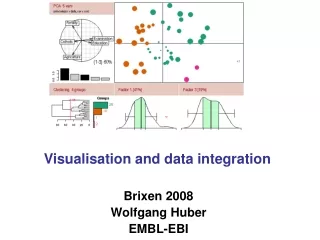
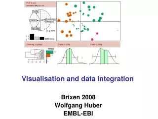
Visualisation and data integration. Brixen 2008 Wolfgang Huber EMBL-EBI. Overview. Visualisation 1-dim. data: distributions 2-dim. data: scatterplots 3-dim. data: pseudo-3D displays a few more than 2-dim: colours, drill-down, lattice, parallel coordinates High-dimensional data

Visualisation and data integration
E N D
Presentation Transcript
Visualisation and data integration Brixen 2008 Wolfgang Huber EMBL-EBI
Overview • Visualisation • 1-dim. data: distributions • 2-dim. data: scatterplots • 3-dim. data: pseudo-3D displays • a few more than 2-dim: colours, drill-down, lattice, parallel coordinates • High-dimensional data • Data integration • Along genomic coordinates • By "gene" identifiers
Univariate data • Suppose you samples of univariate measurements: • Set 1: 0.81, 3.36, 6.84, 9.36, 2.91, 1.81, 5.07, 1.26, 7.89, 9.15, 3.30, 4.35, … • Set 2: 6.57, 5.92, 5.78, 6.63, 5.38, 5.98, 6.30, 6.34, 6.45, 6.57, 6.40, 5.89, … • How do you visualize that?
Density estimation R function density: (i) disperses the mass of the empirical distribution over a regular grid of >= 512 points, (i) uses the fast Fourier transform to convolve this approximation with a discretized version of the kernel, (iii) uses linear approximation to evaluate the density at the specified points.
Empirical Cumulative Distribution Function: ecdf • x = rnorm(12) • Fn = ecdf(x) • plot(Fn) • Fn(x) is the fraction of data points with a value ≤ x.
Discussion: boxplot, histogramme, density, ecdf • Boxplot makes sense for unimodal distributions • Histogramme requires definition of bins (width, positions) and can create visual artifacts esp. if the number of data points is not large • Density requires the choice of bandwidth; plot tends to obscure the sample size (i.e. the uncertainty of the estimate) • ecdf does not have these problems; but is more abstract and its interpretation requires some training. Good for reading off quantiles and shifts in location in comparative plots; OK for detecting differences in scale; less good for detecting multimodality.
Impact of non-linear transformation on the shape of a density • y: sample from a mixture of two log-normal distributions • kernel density estimates
Univariate measurements from a 96-well microtitre plate experiment • Detection of edge effects • Replicate reproducibility package prada
package splots
3D rgl package demo
Using colors • Different requirements for line colours than for area colours • Avoid artefacts related to human perception • Many people are red-green color blind • Lighter colours tend to make areas look larger than darker colors, thus colors of equal luminance should be chosen for graphics with large filled areas or where perception of area is important.
Light Emission Spectra The spectral density of light waves is a function of wavelength l. This function space is infinite dimensional. Spectrometers measure such densities on a dense sampling grid. But our eyes are not a spectrometer.
How human colour vision is thought to have evolved • perception of light/dark by cone cells (monochrome; sensitive to yellow and green wavelengths) • Evolution (pre-mammal) of a second class of cone cells with sensitivity for blue-violet wavelengths. In combination with 1, allows to see contrasts along a "yellow/blue" axis (usually associated with our notion of warm/cold colors) • Primates, 30 Ma ago: specification of the yellow/green cones into two classes: one more sensitive to green, one more to red, allowing to see contrasts in that part of the spectrum (helpful for assessing the ripeness of fruit) • Although the space of all possible wavelength spectra is infinite-dimensional, we perceive them as a 3-dimensional signal
Note: genes for the red and green receptors are on the X-chromosome
RGB color space • Motivated by computer screen hardware
Color palettes based on the extremes of the RGB cube hurt the eyes > pie(rep(1,8), col=1:8)
HSV color space • Hue-Saturation-Value (Smith 1978) Vmin: black (one point) Vmax: a planar area of fully saturated colours, with white in the centre wikipedia
HSV color space • GIMP colour selector linear or circular hue chooser and a two-dimensional area (usually a square or a triangle) to choose saturation and value/lightness for the selected hue
perceptual colour spaces • However, human perception of colour corresponds neither to RGB nor HSV coordinates, and neither to the physiological axes light-dark, yellow-blue, red-green • Rather to polar coordinates in the colour plane (yellow/blue vs. green/red) plus a third light/dark axis. Perceptually-based colour spaces try to capture these perceptual axes: • 1. hue (dominant wavelength) • 2. chroma (colorfulness, intensity of color as compared to gray) • 3. luminance (brightness, amount of gray)
The problem with HSV colours HSV HCL Zeileis and Hornik
CIELUV and HCL • Commission Internationale de l’ Éclairage (CIE) in 1931, on the basis of extensive colour matching experiments with people, defined a “standard observer” who represents a typical human colour response (response of the three light cones + their processing in the brain) to a triplet (x,y,z) of primary light sources (in principle, this could be monochromatic R, G, B; but CIE choose something a bit more subtle) • 1976: CIELUV and CIELAB are perceptually based coordinates of colour space. • CIELUV (L, u, v)-coordinates is prefered by those who work with emissive colour technologies (such as computer displays) and CIELAB by those working with dyes and pigments (such as in the printing and textile industries)Ihaka 2003
HCL colours • (u,v) = chroma * (cos h, sin h) • L the same as in CIELUV, (C,H) are simply polar coordinates for (u,v) • 1. hue (dominant wavelength) • 2. chroma (colorfulness, intensity of color as compared to gray) • 3. luminance (brightness, amount of gray)
So now we know everything about how to specify colours with three coordinates - but which ones do we want to use?
Albert Munsell (1858-1918) divided the circle of hues into 5 main hues — R, Y, G, B, P (red, yellow, green, blue and purple). Value, Chroma: ranges divided into 10 equal steps. E.g. R 4/5 = hue of red with a value of 4 and a chroma of 5.
Munsell Colour System Albert Munsell (1858-1918) divided the circle of hues into 5 main hues — R, Y, G, B, P (red, yellow, green, blue and purple). Value, Chroma: ranges divided into 10 equal steps. E.g. R 4/5 = hue of red with a value of 4 and a chroma of 5.
Balance • The intensity of colour which should be used is dependent on the area that that colour is to occupy. Small areas need to be much more colourful than larger ones. • Choose colours centered on a mid-range or neutral value, or; • Choose colours at equally spaced points along smooth paths through (perceptually uniform) colour space: equal luminance and chroma and correspond to set of evenly spaced hues.
sequential qualitative diverging Software RColorBrewer and vcd packages
Qualitative palette From A. Zeileis, Reisensburg 2007
Some useful functions for working with colours • RColorBrewer • display.brewer.all show all palettes • brewer.pal choose one particular palette • RColorBrewer • colorRamp, colorRampPalette interpolate • vcd • sequential_hcl, diverge_hcl, rainbow_hcl palettes • ... and avoid R's default colours
Drilldown Display an overview of the data, and allow the user to interactively investigate details. Little support to do this in R graphics / using R callbacks directly (but see Simon's talk on Friday). It is simple to produce pre-computed drilldownable displays that can be viewed using a webbrowser or PDF reader (nice for collaborations). file:///C:/Documents%20and%20Settings/huber/Desktop/tooltips
Trellis graphics • a framework for the visualization of multivariable data. Its implementation for R is in the package lattice. • Panels are laid out into rows, columns, and pages (reminiscent of a garden trelliswork). On each panel of the trellis, a subset of the data is graphed by a display method such as a scatterplot, curve plot, boxplot, 3-D wireframe, normal quantile plot, or dot plot. Each panel shows the relationship of certain variables conditional on the values of other variables.
Trellis frame or structure of latticework used as a support for growing vines or plants.
Data from an agricultural field trial to study the crop barley. • At six sites in Minnesota, ten varieties of barley were grown in each of two years. • The data are the yields for all combinations of site, variety, and year, so there are 6 x 10 x 2 = 120 observations. • Each panel in the figure displays the 20 yields at a single site. • Note the data for Morris - reanalysis in the 1990s using Trellis revealed that the years had been flipped!