Probability Functions and Random Variables

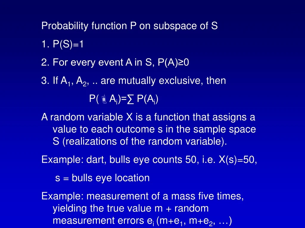
Probability function P on subspace of S P(S)=1 For every event A in S, P(A)≥0 If A1, A2, .. are mutually exclusive, then P(Ai)=∑ P(Ai) A random variable X is a function that assigns a value to each outcome s in the sample space S (realizations of the random variable). Example: dart, bulls eye counts 50, i.e. X(s)=50, s = bulls eye location Example: measurement of a mass five times, yielding the true value m + random measurement errors ei (m+e1, m+e2, …)

Probability Density Function (PDF), fX(x) The relative probability of realizations for a random variable P(X≤a)=∫ fX(x)dx ∫ fX(x)dx = 1 PDF for common functions: Uniform random variable on [a,b]: fU(x)=1/(b-a), a≤x≤b; 0, x<a or x>b a - - -

PDF for common functions: 2. Normal (Gaussian) function: fN(x)=1/√2 exp(-0.5(x-)2/2) N(2) normal distribution 3. Exponential function: fexp(x)= exp(-x), x≥0; 0, x<0

4. Double-sided Exponential function: fdexp(x)=[1/(23/2] exp(-√2|x-) 5.  function: f  x 0.5-1 exp(-x/2) with xx-1e-d n independent variable with standard normal distributions, Z=∑Xi2 is arandom variable with =n degrees of freedom.  0

6 . Student's t distribution with  degrees of freedom: ft(x)/2) 1/√ (1+x2/)-(+1)/2 with xx-1e-d Approaches a standard normal distribution for large number of degrees of freedom Cumulative distribution functions (CDF): FX(a)=P(X≤a)=∫ fX(x)dx P(a≤X≤b) = ∫f(x)dx a - b a

Characterization of PDF’s: Expected value of random variable x: E[X] = ∫ xfX(x)dx, E[g(X)] = ∫ g(x)fX(x)dx Peak of distribution: XML (maximum likelihood) Variance: Var(X)=X2 = E[(X-x)2] = E[X2]-X2 = ∫ (x-x)2 fX(x)dx, x=√Var(X) Variance measures the width of PDF’s. Wide PDF’s indicate noisy data, narrow indicate relatively noise-free data.  -  -  -

Joint PDF’s: The joint PDF can quantify the probability that a set of random variables will take on a given value. f(X≤a,Y≤b)= ∫ ∫ f(x,y)dydx Expected value for joint PDF: E[g(X,Y)]=∫ ∫ g(x,y)f(x,y)dydx If X and Y are independent, f(x,y)=fX(x)fY(y) a - b -  -  -

Covariance of X and Y with Joint PDF: Cov(X,Y)=E[(X-E[X])(Y-E[Y])]=E[XY]-E[X]E[Y] X and Y independent, E[XY]=E[X]E[Y] and Cov(X,Y)=0 Covariance of a variable with itself = variance If Cov(X,Y)=0, X and Y are called uncorrelated Correlation of X and Y (X,Y)=Cov(X,Y)/√Var(X) Var(Y) (correlation is a scaled covariance)

Model covariance matrix cov(m): The general model mest=Md + v has covariance matrix M[cov d]MT (B.64) The least-squares solution mest=[GTG]-1GTd has covariance matrix [cov m] = [GTG]-1GT [cov d] ([GTG]-1GT)T If data is uncorrelated and has equal variance d2 then [cov m] = d2 [GTG]-1

More on Gaussian (Normal) distributions: Central limit theorem: Let X1, X2, …, Xn be independent and identically distributed random variables with finite expected value  and variance 2. Let Zn=[X1+X2+..+Xn-n/√n In the limit as n approaches infinity, Zn approaches the standard normal distribution Thus many summed variables in nature are normal distributions, thus LS solutions OK

Means and confidence intervals: Given noisy measurements m1, m2, .., mn Estimate the true value m and the uncertainty of the estimate. Assume errors are independent and normally distributed with expected value 0 and some unknown standard deviation  Compute average mave=[m1+m2+..+mn/n s=[∑ (mi-mave)2]1/2/n-1 n i=1

Sampling Theorem: Independent, normally distributed measurements, with expected value m and standard deviated , the random quantity t = (m-mave)/s√n has a Student’s t distribution with n-1 degrees of freedom. If the true standard deviation  is known, we are dealing with a standard normal distribution. The t distribution converges toward the normal distribution for large n

Confidence intervals: Probability that one realization falls within a specified distance of the true mean Let tn-1,0.975 = 97.5 percentile of t distribution tn-1,0.025 = 2.5 percentile of t distribution P(tn-1,0.975 ≤m-mave/(s/√n) ≤tn-1,0.025)=0.95 P(tn-1,0.975 s/ √n ≤m-mave ≤tn-1,0.025 s/√n )=0.95 95% confidence interval Due to symmetry: mave-tn-1,0.975 s/ √n to mave+tn-1,0.975 s/ √n

Confidence intervals related to the  - PDF’s with large  will have large CI, and vice versa Gaussian PDF, the 68% CI is 1 wide and the 95% CI is 2 wide If a particular Gaussian random variable has =1, and if a realization of that variable is 50, there is a 95% chance that the mean of that random variable lies between 48 and 52

Example B.12 illustrates the case where  is estimated If  is known (rarely the case), we have a normal distribution. We can use the t-distribution with an infinite # of observations. E.g., 16 obs, m estimated to be 31.5. is known to be 5. Estimate 80% CI for m. mave-k ≤ m ≤ mave+k k=1.282 x 5/√16 = 1.6 31.5-1.6 ≤ m ≤ 31.5+1.6

Statistical Aspects of LS: PDF for Normal Distribution: fi(di|m)=1/√2 exp(-(di-(Gm)i)2/22) Maximum likelihood function L(m|d) is the product of all individual probability functions: L(m|d)=f1(d1|m)*f2(d2|m)* … * fm(dm|m) Idea: Maximize L(m|d) Maximize log{L(m|d)} Minimize - log{L(m|d)} Minimize -2 log{L(m|d)} min ∑ [di-(Gm)I]2/2 Aside from the 1/2 factor, we have the LS solution

min ∑ [di-(Gm)I]2/2 W=diag(1/1, 1/2, …,1/m) Gw=WG dw=Wd Gwm=dw mL2=[GwTGw)-1 GwTdw ||dw-Gwmw||22= ∑ [di-(Gm)I]2/2 obs2 = ∑ [di-(Gm)I]2/2 obs2 has a2 distribution with m-n degrees of freedom

The probability of finding a 2 value as large or larger than the observed value is p=∫ f2(x)dx p-value test With correct model and independent error, the p-values will be uniformly distributed between 0 and 1. Near-0 or near-1 p-values indicates problems (incorrect model, underestimation of data errors, unlikely realization)  obs2

Multivariate normal distribution Random variables X1, …, Xn have a multivariate normal distribution, then the joint PDF is (B.61) f(x)=(2)-n/2 (det[C])-1/2 exp[-(x-)TC-1(x-)/2] Ci,j=Cov(Xi,Xj)

Eigenvalues and eigenvectors Axl x (A-lIx=0 det (A-lI) = 0 The roots l are the eigenvalues

SVD G=USVT U (m x m) orthogonal spanning data space V (n x n) orthogonal spanning model space S (m x n) eigenvalues along diagonal Let rank(G)=p G=[Up U0] [Sp 0;0 0] [Vp V0]T = UpSpVpT G+=VpSp-1UpT = Generalized Inverse (pseudoinverse) m+=G+d=VpSp-1UpT d = pseudoinverse solution Since Vp-1=VpT and Up-1=UpT (A.6)

SVD G=USVT U (m x m) orthogonal spanning data space V (n x n) orthogonal spanning model space S (m x n) eigenvalues along diagonal Rank(G)=p Theorem A.5: N(GT)+R(G)=Rm, i.e. p columns of Up form an orthonormal basis for R(G) columns of U0 form an orthonormal basis for N(GT) p columns of Vp form an orthonormal basis for R(GT) columns of V0 form an orthonormal basis for N(G)

Properties of SVD G=USVT N(G) and N(GT) are trivial (only null vector): Up=U, Vp=V square orthogonal matrices, and UpT=Up-1 and VpT=Vp-1 G+=VpSp-1UpT = (UpSpVpT)-1 = G-1 (inverse for full rank matrix, m=n=p). Unique solution, data are fit exactly.

Properties of SVD G=USVT 2. N(G) is nontrivial (model, V); N(GT) is trivial (data, U) UpT=Up-1 and VpTVp=Ip Gm+=GG+d=UpSpVpTVpSp-1UpTd=UpSpIpSp-1UpTd=d i.e. the data are fit exactly an LS solution, but nonuniquely due to the nontrivial model null space m=m++m0 =m++∑ iV.,I ||m||22=||m+||22 +∑ i ≥||m+||22 -> minimum length solution n i=p+1 n i=p+1

Properties of SVD G=USVT 3. N(G) is trivial (model, V); N(GT) is nontrivial (data, U) Gm+=GG+d=UpSpVpTVpSp-1UpTd=UpUpTd = projection of d onto R(G), I.e. the point in R(G) that is closest to d, m+ is LS solution to Gm=d. If d is in R(G), m+ will be solution to Gm=d. Solution is unique but does not fit data exactly i.e. the data are fit exactly an LS solution, but nonuniquely due to the nontrivial model null space m=m++m0 =m++∑ iV.,I ||m||22=||m+||22 +∑ i ≥||m+||22 -> minimum length solution n i=p+1 n i=p+1

Properties of SVD G=USVT 4. N(G) is nontrivial (model, V); N(GT) is nontrivial (data, U) p < (m,n) Gm+=GG+d=UpSpVpTVpSp-1UpTd=UpUpTd = projection of d onto R(G), I.e. the point in R(G) that is closest to d, m+ is LS solution to Gm=d. i.e. LS solution to minimum norm, as case 2)

Properties of SVD G=USVT - Always exists - LS or minimum length - Properly accommodates the rank and dimensions of G - Nontrivial model null space m0 the is heart of the problem -> - Infinite # of solutions will fit the data equally well, since components of N(G) have no effect on data fit, I.e., selection of a particular solution requires a priori constraints (smoothing, minimum length) - Nontrivial data space are vectors d0 that have no influence on m+. If p<n, there are an infinite # of data sets that will produce the same model

Properties of SVD - covariance/resolution Least squares solution is unbiased: min ∑ [di-(Gm)I]2/2 W=diag(1/1, 1/2, …,1/m) Gw=WG, dw=Wd, Gwm=dw mL2=[GwTGw]-1 GwTdw ||dw-Gwmw||22= ∑ [di-(Gm)I]2/2 E[mL2]=E[(GwTGw)-1 GwTdw] = (GwTGw)-1 GwT E[dw]= (GwTGw)-1 GwT dwtrue = (GwTGw)-1 GwT Gwmtrue = mtrue

Properties of SVD - covariance/resolution Generalized inverse not necessarilyunbiased: E[m+]=E[G+d] = G+E[d]= G+Gmtrue = Rmmtrue Bias= E[m+]-mtrue =Rmmtrue-mtrue = (Rm-I)mtrue = VpVpT-VVTmtrue=-V0V0T mtrue I.e., as p increasees Rm->I Cov(mL2)=2(GTG)-1 Cov(m+)=G+[Cov(d)]G+T = G+G+T =VpSp-2VpT = ∑ V.,i V.,iT/i2 I.e., as p increases, Rm->I: bias decreases while variance increases…! P I=1

Model resolution Rm -> I: increasing resolution Resolution test: multiply Rm onto a particular model, fx a spike model, with one element 1 and the rest 0, picks out the corresponding column of Rm Data resolution D+=Gm+ = GG+d = Rdd Rd=UpSpVpTVpSp-1UpT=UpUpT p=m -> Rd=I, d+=d p<m -> Rd<>I, m+ doesn’t fit data exactly Rm, Rd can be assessed during design of experiment

Instabilitites of SVD Small eigenvalues -> m+ sensitive to small amounts of noise Small eigenvalues maybe indistinguishable from 0 Possible to remove small eigenvalues to stabilize solution -> Truncated SVD, TSVD Condition number cond(G)=s1/sk

Probability Functions and Random Variables