Download
1 / 31
320 likes | 448 Views
A New Recombination Lower Bound and The Minimum Perfect Phylogenetic Forest Problem. Yufeng Wu and Dan Gusfield UC Davis COCOON’07 July 16, 2007. Suffix. Prefix. 11000. 0000001111. Breakpoint. Recombination.

E N D
A New Recombination Lower Bound and The Minimum Perfect Phylogenetic Forest Problem Yufeng Wu and Dan Gusfield UC Davis COCOON’07 July 16, 2007
Suffix Prefix 11000 0000001111 Breakpoint Recombination • Recombination: one of the principle genetic forces shaping sequence variations within species • Two equal length sequences generate a third new equal length sequence during meiosis. 110001111111001 000110000001111
1 0 0 1 1 1 Ancestral Recombination Graph (ARG) 00 Mutations 00 Recombination 10 01 10 11 01 00 Network, not tree! Assumption:at most one mutation per site
A Min ARG for Kreitman’s data ARG created by SHRUB
Minimizing Recombination • Given enough recombinations, any set of sequences can be trivially derived on an ARG. • Problem: Given a set of sequences M, construct an ARG that derives M using one mutation per site, and the minimum number of recombinations (Rmin). • NP-hard (Wang, et al 2001, Semple et al.). • Efficiently computed Lower bounds on Rmin exist.
000 00 00 100 10 10 Empty. One type-3 operation 010 01 01 011 01 History Bound (Myers & Griffiths 2003) M 000 100 010 011 111 • Iterate the following operations • Remove a column with a single 0 or 1 • Remove a duplicate row • Remove any row • History bound: the minimum number of type-3 operations needed to reduce the matrix to empty
Graphical interpretation of history bound (HistB) • Each operation corresponds to an operation that decomposes the optimal, but unknown ARG. • Removing an exposedrecombination node in the ARG corresponds to a single type-3 operation. So when decomposing the optimal ARG, the number of recombination nodes => number of corresponding type-3 operations. • However, not all type-3 operations correspond to removing a recombination node. • Since the optimal ARG is unknown, the history bound is the minimum number of type-3 operations needed to make the matrix empty.
a: 00010 b: 10010 4 M c: 00100 3 d: 10100 e: 01100 f: 00101 1 g: 00101 Operations on M correspond to operations on the optimal ARG s p a: 00010 2 c: 00100 b: 10010 d: 10100 2 5 e: 01100 g: 00101 f: 00101
12345 a: 00010 b: 10010 4 c: 00100 3 d: 10100 e: 01100 f: 00101 1 s Type-2 operation p a: 00010 2 c: 00100 b: 10010 d: 10100 2 5 e: 01100 f: 00101
134 a: 001 b: 101 4 c: 010 3 d: 110 e: 010 f: 010 1 s Type-1 operations p a: 001 2 c: 010 b: 101 d: 110 e: 010 f: 010
134 a: 001 b: 101 4 c: 010 3 d: 110 1 Type-2 operations s p a: 001 2 c: 010 b: 101 d: 110
134 a: 001 b: 101 4 c: 010 3 1 Type-3 operation a: 001 c: 010 b: 101 Then three more Type-1 operations fully reduce M and the ARG.
History bound • Initially required trying all n! permutations of the rows to choose the type-3 operations. • The bound can be computed by DP in O(2n) time (Bafna, Bansal). • On datasets where it can be computed, the history bound is observed to be higher than (or equal to) all studied lower bounds (about ten of them). • There is nostatic definition for what the history bound is -- it is only defined by the algorithms that compute it! The work in this paper comes out of an attempt to find a simple static definition.
Why a static definition matters • We want a definition of what is being computed, independent of how it is computed, so that we can reason about it and find alternative ways to compute or approximate it. • For example, with no static definition of the history bound, we don’t know how to formulate an integer linear program to compute it.
Perfect Phylogeny Only one mutation per site allowed. sites 12345 00000 1 4 Site mutations on edges 3 00010 The tree derives the set M: 10100 10000 01011 01010 00010 starting from 00000 2 10100 5 10000 01010 01011
After removing recombination edges, four trees result. Intro. to Forest Bound: Decompose an Optimal ARG to A Forest of Trees, removing recombination edges The number of trees is precisely the number of recombinations plus one An ARG with three recombinations
Idea behind the Forest Bound (FB) Each tree created in this way contains at most one occurrence of any site, and each site occurs in at most one of the trees. So the trees form a forest of related perfect phylogenies.
Forest Bound Given a set of sequences M, partition M into the fewest subsets so that each subset of sequences can be derived on a tree, where each site occurs at mostonce in the forest of trees. The number of trees, minus one, is a valid lower bound on Rmin.
Comparing the Forest Bound (FB) to: • History Bound (HistB) • Optimal Haplotype Bound (OhapB): The currently best lower bound that can be computed in practice for biological data. • Theorem: On any data, OhapB <= FB <= HistB On some data, OhapB < FB < HistB Thus the FB is the highest lower bound with a static definition.
First, define the Haplotype Lower Bound (S. Myers, 2003) • Rh = Number of distinct sequences (rows) - Number of distinct sites (columns) -1 <= minimum number of recombinations needed (folklore) • Before computing Rh, remove any site that is compatible with all other sites. A valid lower bound results - generally increases the bound. • Generally Rh is really bad bound, often negative, when used on large intervals, but Very Good when used as local bounds in the Composite Method. Myers implemented the method in a program called RecMin, which was a huge advance, generally three times higher than the prior best lower bound method. • The composite method can be used with any lower bound method and the better the initial lower bounds, the better the composite result.
Then, the Subset Bound (Myers) • Let S be a subset of sites, and Rh(S) be the haplotype bound computed on the sequences restricted to S. Rh(S) is a valid lower bound on Rmin. • Optimal Haplotype Bound (OhapB) is the maximum Rh(S) over all subsets of sites. • Practical computation of OhapB via ILP was studied in (SWG 2005) and exploited in the program Hapbound. Hapbound gives provably better bounds than RecMin.
0 0 0 1 Rh = 4 – 2 – 1 = 1 1 0 1 1 Now, the Optimal Haplotype Bound (OhapB) • OhapB is the maximum haplotype bound over any subset of columns. • NP-hard (Bafna & Bansal, 2005) • Efficiently computed in practice (Song, Wu, Gusfield 2005) Rh = 4 – 3 – 1 = 0
Forest Bound (FB) is Higher than Haplotype Bound (Rh) Rh = number distinct rows – number distinct columns – 1 = 5 -- 5 --1 = --1 10001 00010 Steiner nodes FB = 2 s4 s1 s5 s2 00100 s3 01101 11011
FB >= Rh FB obtained from all the data M is >= FB obtained from a subset of the columns, so assume all columns in M are distinct. FB = # trees in the FB -- 1 = # nodes -- # edges -- 1 in the forest = # leaves + # Steiner nodes -- # columns -- 1 = # rows + # Steiner nodes -- # columns -- 1 >= # distinct rows -- # columns-- 1 = Rh
Optimal subset of columns Ms s2 s3 s5 s2 s3 s5 Forest Bound is Higher than Optimal Haplotype Bound Input matrix M F(Ms) Rh(Ms) (i.e. the optimal haplotype bound).
s2, s3, s5. Cleanup s5 s5 s3 s2 s2 A legal forest for the subset data! A legal forest with 3 trees for the subset Number of Trees after Taking Subset of Columns Also, taking subsets can not increase the number of trees, and so FB(M) FB(Ms). So, FB(M) FB(Ms) Rh(Ms), so FB OhapB s5 s1 s3 s3 s2 s4 s6 Minimum forest with 3 trees for entire data
FB <= HistB The decomposition of the optimal ARG, directed by the operations of computing the history bound, creates a forest of HistB + 1 trees, where each site occurs at most once, in at most one tree. So FB <= HistB.
Computing the Forest Bound is NP-Hard • Optimal haplotype bound is quite good, but NP-hard to compute. • If the forest bound can be efficiently computable, we do not need to use optimal haplotype bound at all. • Unfortunately, the forest bound is NP-hard to compute. • Reduction from Exact-cover-by-3 sets.
Binary sequences on a hypercube Two sequences from different sets are far apart, and would need two many mutations to connect, thus can not belong to the same tree. Sequences corresponding to same element in two sets need same mutation and thus can not be both chosen. NP-hardness Proof for the Minimum Perfect Phylogenetic Forest Problem 3-Sets Sequences corresponding to the same set form a perfect phylogeny with a single novel sequence (not in input) {1,3,5} {1,2,4} {2,4,6}
Integer Programming Formulation for the Forest Bound • For sequences with m sites, consider the hypercube all possible 2m sequences. • Minimizing F is equivalent to reducing the number of Steiner nodes in the forests. • We also need to ensure the edge linking two nodes in a tree is only labeled with columns that do not appear in other trees. • Can easily incorporate the missing data in the input. • The IP formulation has exponential size, but practical when the number of columns is relatively small.
Empirical Results • On random generated dataset with 15 rows and 7 columns, FB > OhapB on 10% of the data. On more biological meaningful data (generated with simulation program ms), however, OhapB= FB more often. • On dataset generated by ms with missing entries, FB is more often outperforms an approximate optimal Rh bound: • 30 rows and 7 columns and 30% missing entries: FB was strictly larger in 8% of the data. • When the level of missing entries is lower, the approx. OhapB matches the FB more often.