Download

1 / 15
150 likes | 170 Views
1-2. Introduction to Parent Functions. Warm Up. Lesson Presentation. Lesson Quiz. Holt McDougal Algebra 2. Holt Algebra 2. Warm Up 1. For the power 3 5 , identify the exponent and the base. Evaluate. 2. 3. f (9) when f ( x )=2 x +. exponent: 5; base: 3. 21. Objectives.

E N D
1-2 Introduction to Parent Functions Warm Up Lesson Presentation Lesson Quiz Holt McDougal Algebra 2 Holt Algebra 2
Warm Up 1. For the power 35, identify the exponent and the base. Evaluate. 2. 3.f(9) when f(x)=2x + exponent: 5; base: 3 21
Objectives Identify parent functions from graphs and equations. Use parent functions to model real-world data and make estimates for unknown values.
Similar to the way that numbers are classified into sets based on common characteristics, functions can be classified into families offunctions. The parent function is the simplest function with the defining characteristics of the family. Functions in the same family are transformations of their parent function.
Helpful Hint To make graphs appear accurate on a graphing calculator, use the standard square window. Press ZOOM , choose 6:ZStandard, press again, and choose 5:ZSquare. ZOOM ZOOM
Example 1A: Identifying Transformations of Parent Functions Identify the parent function for g from its function rule. Then graph g on your calculator and describe what transformation of the parent function it represents. g(x) = x – 3 g(x) = x – 3 is linear x has a power of 1. The linear parent function ƒ(x) = x intersects the y-axis at the point (0, 0). Graph Y1 = x – 3 on the graphing calculator. The function g(x) = x – 3 intersects the y-axis at the point (0, –3). So g(x) = x – 3 represents a vertical translation of the linear parent function 3 units down.
Example 1B: Identifying Transformations of Parent Functions Identify the parent function for g from its function rule. Then graph on your calculator and describe what transformation of the parent function it represents. g(x) = x2 + 5 g(x) = x2 + 5 is quadratic. x has a power of 2. The quadratic parent function ƒ(x) = x intersects the y-axis at the point (0, 0). Graph Y1 = x2 + 5 on a graphing calculator. The function g(x) = x2 + 5 intersects the y-axis at the point (0, 5). So g(x) = x2 + 5 represents a vertical translation of the quadratic parent function 5 units up.
Check It Out! Example 1a Identify the parent function for g from its function rule. Then graph on your calculator and describe what transformation of the parent function it represents. g(x) = x3 + 2 g(x) = x3 + 2 is cubic. x has a power of 3. The cubic parent function ƒ(x) = x3 intersects the y-axis at the point (0, 0). Graph Y1 = x3 + 2 on a graphing calculator. The function g(x) = x3 + 2 intersects the y-axis at the point (0, 2). So g(x) = x3 + 2 represents a vertical translation of the quadratic parent function 2 units up.
It is often necessary to work with a set of data points like the ones represented by the table below. With only the information in the table, it is impossible to know the exact behavior of the data between and beyond the given points. However, a working knowledge of the parent functions can allow you to sketch a curve to approximate those values not found in the table.
Example 2: Identifying Parent Functions to Model Data Sets Graph the data from this set of ordered pairs. Describe the parent function and the transformation that best approximates the data set. {(–2, 12), (–1, 3), (0, 0), (1, 3), (2, 12)} The graph of the data points resembles the shape of the quadratic parent function ƒ(x) = x2. The quadratic parent function passes through the points (1, 1) and (2, 4). The data set contains the points (1, 1) = (1, 3(1)) and (2, 4) = (2, 3(4)). The data set seems to represent a vertical stretch of the quadratic parent function by a factor of 3.
Check It Out! Example 2 Graph the data from the table. Describe the parent function and the transformation that best approximates the data set. The graph of the data points resembles the shape of the linear parent function ƒ(x) = x. The linear parent function passes through the points (2, 2) and (4, 4). The data set contains the points (2, 2) = (2, 3(2)) and (4, 4) = (4, 3(4)). The data set seems to represent a vertical stretch of the linear function by a factor of 3.
Consider the two data points (0, 0) and (0, 1). If you plot them on a coordinate plane you might very well think that they are part of a linear function. In fact they belong to each of the parent functions below. Remember that any parent function you use to approximate a set of data should never be considered exact. However, these function approximations are often useful for estimating unknown values.
Cumulative Sales Year Sales (million $) 1 0.6 2 1.8 3 4.2 4 7.8 5 12.6 Example 3: Application Graph the relationship from year to sales in millions of dollars and identify which parent function best describes it. Then use the graph to estimate when cumulative sales reached $10 million. Step 1 Graph the relation. Graph the points given in the table. Draw a smooth curve through them to help you see the shape.
The curve indicates that sales will reach the $10 million mark after about 4.5 years. Example 3 Continued Step 2 Identify the parent function. The graph of the data set resembles the shape of the quadratic parent function f(x) = x2. Step 3 Estimate when cumulative sales reached $10 million.