Download
1 / 47
470 likes | 751 Views
View-dependent Adaptive Tessellation of Spline Surfaces. Jatin Chhugani & Subodh Kumar Johns Hopkins University. Motivation. Why use Splines? CAD/CAM , Entertainment Industry Medical Visualization Examples Submarines Animation Characters Human body especially the heart and brain.

E N D
View-dependent Adaptive Tessellation of Spline Surfaces Jatin Chhugani & Subodh Kumar Johns Hopkins University
Motivation Why use Splines? • CAD/CAM , Entertainment Industry • Medical Visualization • Examples • Submarines • Animation Characters • Human body especially the heart and brain
Splines • Non-Uniform Rational B-Spline (NURBS) • Bezier patch (rational) Degree m x n Domain space (u, v) [0,1] x [0,1] For 0 i m, 0 j n, Control points : pij Weights: wij
m n wijpij Bmi(u) Bnj (v) i=0 j=0 F(u,v) = m n wij Bmi(u) Bnj (v) i=0 j=0 where Bernstein function Bni (t) = t i (1- t)n-i
Rendering Splines • Ray tracing • J. Kajiya, T. Nishita et al., J. Whitted • Pixel level surface subdivision • E.Catmull, M. Shantz et al. • Scan-line based • J. Blinn, J. Lane et al., J. Whitted • Polygonal Approximations • Forward (static) • Backward (dynamic)
Forward Technique • View-dependent tessellation • Incremental triangulation Backward Technique • Pre-tessellate patches densely • Apply polygon simplification
Forward Technique Advantage • Allows arbitrary precision Disadvantage • Significant computation overhead Backward Technique • Advantage • Low run-time computation • Disadvantages • Large storage requirement • Upper limit on detail of the model
Our Approach • Hybrid of backward and forward techniques • Pre-compute domain samples • Select samples and triangulate dynamically • Generate additional detail when necessary
Domain Space Tessellation • Uniform Tessellation • Adaptive Tessellation
Uniform Tessellation Domain Space
Uniform Tessellation • Fast • Step size computation • Triangulation • Over-tessellation • Triangle Rendering Bottleneck
Adaptive Tessellation Domain Space
Adaptive Tessellation • Generates triangles only where needed • Inefficient • Many ‘stopping test’ computations • Triangulation algorithm not simple
Basic Idea • Pre-sample adaptively to some precision • Maintain samples in ‘order of importance’ • More importance in the areas of high curvature • At rendering time • Select samples • Triangulate • If higher precision needed • Perform uniform tessellation
Pre-Sampling Choose samples on each patch
Questions: #1 For a predefined deviation (between the surface and its triangulation) threshold, what is the minimum number of points required on a patch for a given position and orientation of the patch? And where? Computationally Intractable
Questions: #2 Is there a correlation between these points as the viewing parameters change? Not Always.
Deviation = Δ0Deviation = Δ1 (< Δ0) No common points (except the end points) Figure 1 Figure 2
Heuristic Given a triangulation of a surface that deviates by more than Δ, add samples at the points of highest deviation until the resulting deviation is less than Δ.
Pre-Sampling 1 2 3 4 Domain Space
Pre-Sampling 1 2 Point A Point B 3 4 Point of maximum object space deviation for a triangle
Pre-Sampling 1 2 5 3 4 Domain Space
Pre-Sampling 1 2 C 5 D B A 3 4 Point of maximum object space deviation for a triangle
Pre-Sampling 1 2 5 6 3 4 Domain Space
What is stored ? • Ordered set of (u,v) pairs • by decreasing deviation • Deviation in object space • i.e., deviation after the sample is added • 3-d Vertex • optional
Rendering Time Algorithm Given screen space deviation bounds
Scaling Factor for a patch Scaling Factor for a vector at point P = Minimum ratio of the length of the vector to its projected length on the image plane. Q Ratio = Q P P Eye Image Plane
Scaling Factor for a patch • Pre-processing • Partition space • For each patch, use the partition containing it • If too many partitions for a patch, subdivide patch • Run-time (for each frame) • Compute the scaling factor for each partition • Scaling factor a patch is that of its partition
Runtime Algorithm • Compute max allowable deviation (say c) • Let p = max deviation in current triangulation • if (c > p) • delete domain samples having deviation less than c • update triangulation
Example P1 P2 P3 P4 P5 P6 P7 P8 UV Values 26 24 21 19 14 13 6 3 Deviation Here p = 3 Let c = 20 UV Values P1 P2 P3 P4 26 24 21 19 Deviation
Runtime Algorithm • if (c < p) • add domain samples having deviation greater than c • update triangulation • if pre-computed set is exhausted • Uniformly tessellate triangles having deviation greater than c
Adaptive + Uniform Tessellation Pre-computed Samples Computed at run time to uniformly tessellate triangles having deviation greater than threshold
Potential Problem Cracks in the model
Boundary Curve Crack v u Samples on the boundary curve for left patch Samples on the boundary curve for the right patch Different samples on adjacent boundary curves
Crack Prevention • Sample the boundary curves separately from the interior, to prevent cracks in adjacent patches. • Modify the interior patch sampling by deleting points too close to the boundary.
Crack Prevention Boundary Curve v u Samples on the boundary curve for the two adjacent patches Same samples on adjacent boundary curves
Results Model details
Results Pre-sampling Performance
Results Comparison for average number of triangles generated per frame [20]: “Interactive display of large NURBS models” by S. Kumar, D. Manocha and A. Lastra
Results Run-time behavior of our algorithm
Conclusions • Combines forward and backward techniques • Uses adaptive and uniform tessellation • Low triangle count, small memory footprint • Applicable to class of parametric surfaces • Towards real-time spline surface rendering
Acknowledgements • Shankar Krishnan • Lifeng Wang • UBC Modeling group • Alpha 1 Modeling system • National Science Foundation