Applying Computer Based Assessment Using Cognitive Diagnostic Modeling to Benchmark Tests
Applying Computer Based Assessment Using Cognitive Diagnostic Modeling to Benchmark Tests. Terry Ackerman, UNCG Robert Henson, UNCG Ric Luecht, UNCG Jonathan Templin, U. of Georgia John Willse, UNCG. Tenth Annual Assessment Conference


Applying Computer Based Assessment Using Cognitive Diagnostic Modeling to Benchmark Tests
E N D
Presentation Transcript
Applying Computer Based Assessment Using Cognitive Diagnostic Modeling to Benchmark Tests Terry Ackerman, UNCG Robert Henson, UNCG Ric Luecht, UNCG Jonathan Templin, U. of Georgia John Willse, UNCG Tenth Annual Assessment Conference Maryland Assessment Research Center for Education Success University of Maryland, College Park, Maryland October 19, 2010
Overview of talk • Purpose of the study • The Cumulative Effect Mathematics Project • Phase I paper and pencil benchmark test • Q-matrix development • Item writing • Standard setting • Results - Fitting the CDM model • Teacher feedback • Phase II Multistage CDM CAT • Multistage CDM (development and administration) • Future Directions
Purpose We are currently part of the evaluation effort of a locally and state funded project called the Cumulative Effect Mathematics Project. As part of that effort, we are applying cognitive diagnostic modeling (CDM) to a benchmark test used in an Algebra II course in Guilford County, North Carolina. Our goal is to eventually make this a computerized CDM assessment.
Cumulative Effect Mathematics Project The CEMP involves the ten high schools in Guilford County that had the lowest performance on the End-of-Course tests in mathematics. The EOC test is part of the federally mandated accountability test under the No Child Left Behind Legislation. The ultimate goal of the CEMP is to increase mathematics scores at these ten high schools.
Benchmark Testing Currently in North Carolina, teachers follow strict instructional guidelines called a “standard course of study”. These guidelines dictate what objectives and content must be taught during each week. The instruction must “keep moving”. Given this pacing teachers often struggle on how to effectively assess students’ learning to make sure they are prepared to take the End-of-Course Test. This is a very “high-stakes” test because it could have implications for both the student (passing the course) and the teacher (evaluation of his or her effectiveness as a teacher). End- of-Course Test Standard course of study September May
Benchmark Testing One common method of formative assessment is the “benchmark test”. These tests would provide intermediate feedback of what the student has learned so that remediation, if necessary, can be implemented prior to the end-of course test. End- of-Course Test Standard BT Course of BT Study Remediation Remediation
Potential Benefits of using Cognitive Diagnostic Modeling (CDM) on benchmark tests • By constructing the benchmark test to measure attributes with CDMs, several benefits can be realized. • Student information comes in the form at of a profile of skills that the student has mastered and not mastered. • The skills needed to perform well on the EOC are measured directly. • The CDM profile format can diagnostically/prescriptively inform classroom instruction. • The profile can help students better understand their strengths and weaknesses. • When presented in a computerized format there is immediate • feedback provided to the teacher and students.
Models used for Cognitive Diagnosis Many cognitive diagnosis models (CDM) are built upon the work of Tatsouka (1985) and requires one to specify a Q-matrix. For a given test, this matrix identifies which attributes each item is measuring. Thus, for a test containing J items and K attributes the J x K Q-matrix contains elements, qjk, such that Also, instead of characterizing examinees with a continuous latent variable, examinees are characterized with a 0/1 vector/profile, αi , whose elements denote which of the k attributes subject i has mastered.
Example Q-matrix Attribute F is being assessed by items 2 and 5 1= item requires attribute K - Attributes/Skills J - Items Item 6 requires attributes D and E.
Choosing the Attributes We chose to use the attributes as defined by the Department of Public Instruction’s standard course of study’s course objectives and goals • On the EOC students would ultimately be evaluated in relation to these course objectives and goals. • Teachers were already familiar with those definitions and the implied skills
Objectives Retained for our Q-Matrix • 1.03 Operate with algebraic expressions (polynomial, rational, complex fractions) to solve problems • 2.01 Use the composition and inverse of functions to model and solve problems: justify results • 2.02 Use quadratic functions and inequalities to model and solve problems; justify results • a. Solve using tables, graphs and algebraic properties • b. Interpret the constants and coefficients in the context of the problem • 2.04 Create and use best-fit mathematical models of linear, exponential, and quadratic functions to solve problems involving sets of data • a. Interpret the constants, coefficients, and bases in the context of the data. • b. Check the model for goodness-of-fit and use the model, where appropriate, to draw conclusions or make predictions • 2.08 Use equations and inequalities with absolute value to model and solve problems: justify results. • a. Solve using tables, graphs and algebraic properties. • b. Interpret the constants and coefficients in the context of the problem.
The Assessment • After we discussed the concept of a Q-matrix with a group of three Master teachers, we had them write items measuring one or more of the attributes. From this pool of “benchmark” items a pencil and paper assessment was created • These items were then pilot tested and the assessment was refined using traditional CTT techniques • A final form was created and the Q-matrix was further verified by another set of five master teachers.
The Simple Math Example used to verify the Q-matrix Example Test Measuring Basic Math: 2+3-1=? 2/3=? 2*4=? Notice that in this example every item does not require the four skills (add, subtract, multiply, and divide) and so we need to describe which skills are needed to answer each item. The way that we will summarize this information by using a table like the one below. We ask that you simply provide a check (or an “X”) under those skills that would be needed to correctly answer each of the items. Again we provide an example of the final table. We ask that you simply provide a check (or an “X”) under those skills that are needed to correctly answer each of the items.
Generalizabilty study We also conducted a generalizability study to examine the dependability the process of assigning the attributes to the items. The sources of variability included: • Test-Items, Object of Measurement • Raters: Teachers indicating which attributes were required in order to answer items • Attributes Influencing the items (attributes were treated as fixed) In G-theory there is a coefficient for relative decisions (i.e., ranking), g, and one for absolute decisions (i.e., criteria-based),
Dependability of the Q-Matrix • Under our current design (shaded row) the highest dependability coefficients were obtained for objectives 2.01 and 2.08 Dependability of assigning attributes Attributes
The Final Q-Matrix • The average q-matrix complexity is 1.36 • 9 items require 2 attributes • 16 items require 1 attribute • Stem for item 2 • If one factor of f(x) = 12x2 – 14x – 6 is (2x – 3) what is the other factor of f(x) if the polynomial is factored completely.
The LCDM 17 In this particular case we used the Log-linear Cognitive Diagnosis Model ( Henson, Templin, and Willse, 2007). The LCDM is a special case of a log-linear model with latent classes (Hagenaars, 1993) and thus is also a special case of the General Diagnostic Model (von Davier, 2005). The LCDM defines the logit of the probability of a correct response as a linear function of the attributes that have been mastered.
The LCDM Note that the two-attribute LCDM is very similar to a two-factor ANOVA with two main effects and an interaction term 18 Given the simple item, 2+3-1=?, we can model the logit of the probability of a correct response as a function of mastery or non-mastery of the two attributes (addition and subtraction). Specifically,
Standard Setting 19 • Although the LCDM item parameters can be estimated, it was important to define the parameters so that mastery classifications would be consistent with the standards set by the EOC. • In getting these probabilities the standard is set for all possible combinations of mastery. • Thus, we define how a student will be classified in the mastery of each attribute.
Estimating LCDM item parameters using Standard Setting 20 • The teachers we used to verify the Q-matrix also helped us perform a standard setting using a modified Angoff approach. • For each item, teachers were asked to identify what proportion of 100 students who mastered the required attributes and what proportion of 100 students who had not mastered the required attributes would get the item correct. • These proportions were then averaged across raters and used to determine the parameters for each item in the LCDM model.
Example Standard Setting Responses Item 1 (01000) • 1. If f(x) = x2 +2 and g(x) = x – 3 • find . • a. x2 – 6x +11 • b. x2 +11 • c. x2 +x – 1 • d. x3 – 3x2 +2x – 6 P(X=1|Non-master) P(X=1|Master) 21
Example Standard Setting Responses Item 6 (01010) • Determine which of the • following graphs does not represent Y as a linear function of X. 00 10 01 11 P(X=1) 22
Analyses 23 • Based on the teachers’ standard setting responses, the average probability of a correct response was calculated. • These averages are used to compute item parameters. • Specifically, if we know the probabilities associated with each response pattern (based on the teachers’ responses) then we can compute the logit. Therefore we can directly compute the item parameters. For a simplified version having only two attributes the model would like:
We administered the test and then using these fixed parameters as truth, we obtained estimates of the posterior probability that each skill has been mastered. A mastery profile, , was created, i.e., the probabilities. were then categorized as mastery or non-mastery using the rule: Greater than 0.50 equals a master. Less than 0.50 equals a non-master. 24
Example Feedback 01110 25
Example Feedback 11010 26
S’s 1.01 2.01 2.02 2.04 2.08 1 0.8651 0.74150.53030.3925 0.2449 2 0.9820 0.2816 0.9204 0.3647 0.1692 3 0.9792 0.9531 0.9236 0.8814 0.9663 4 0.2045 0.1180 0.4381 0.1200 0.0601 5 0.8447 0.5948 0.3821 0.7483 0.8820 6 0.6573 0.8807 0.5966 0.8628 0.7690 Examinee Posterior Probabilities of Mastery Non Master < .45.45 < Unsure < .55Master >.55 Mrs. Jones Students’ results
1.01 2.01 2.02 Non-master 5 23.8% Non-master 4 19% Non-master 5 23.8% Unsure 1 4.8% Unsure 3 14.3% Unsure 1 4.8% Master 15 71.4% Master 14 66.7% Master 15 71.4% 2.04 2.08 Non-master 3 14.3% Non-master 5 23.8% Unsure 5 23.8% Unsure 1 4.8% Master 13 61.9% Master 15 71.4% Mrs. Jones’ Algebra II class results
Benchmark results were linked to students’ EOC performance. Then for each profile, a mean EOC score was computed. Using this chart we then can indicate for a teacher, which skills will result in the largest gain on the EOC. That is, assume an individual has not mastered any of the three attributes and has a profile of (0,0,0). If he or she mastered attribute 1 the expected EOC gain would be 1 point, if they mastered attribute 2, the gain would be 3 points, and if they mastered attribute 3 the gain would be 4 points. Thus, if time is limited it would be best for this individual to learn attribute 3.
Roadmaps to Proficiency Using the distances between expected increases in EOC scores for each vector additional attribute mastered Templin was able to treat these distances as “strengths of relationship” and use the Social Network Theory software Pajek to create the following “Roadmap to Mastery”.
Road Map to Mastery Mastery of No skills Mastery of all skills
Pathways to EOC attribute Mastery 11010 10010 0 6 12 18 24 EOC test scale
Conversion to a Multistage CAT test We are in the process of converting the benchmark test to a multistage computer adaptive test. To do this we are going to approximate the same procedure that would be used in a traditional CAT. That is, typically in a CAT items are selected to provide the greatest amount of information at the current estimated ability level. To create an analogous approach with diagnostic models we will use an index that is a measure of attribute information.
Multi-stage testing for DCM Currently we are conducting simulation studies and compare the proportion of correct classification of identifying attribute patterns using several different testing scenarios. Initially we are experimenting with three attributes and then will expand the configuration to five attributes. This work combines the work of Henson, et al (2008), Luecht (1997) and Luecht, Brumfield and Breithaupt (2004). Using a pool of 200 generated items and 1000 examinees we are in the process of verifying the success of a multistage CAT format for the CDM. For this comparison we hope to compare three testing scenarios.
Verifying the accuracy of a Multistage CDM CAT Scenario One: Create a 30-item test using Henson’ et al’s db attribute discrimination index. That is, assuming a uniform distribution of ability, 30 items having the highest db values would be selected and the administration to the 1000 examinees would be simulated. Scenario Two, would be to simulate a multistage adaptive CAT. Scenario Three, would be to use Chang’s CAT approach.
Attribute specific item discrimination indices using the Kullbeck-Leibler Information (KLI) In diagnostic modeling instead of using the Fisher information function, the Kullback-Leibler Information (KLI) is used. KLI represents the difference between two probability distributions. Henson, Roussos, Douglas and He (2008) developed an index, dbthat describes the discrimination for a specified distribution of attribute patterns. This index can be aggregated for multiple items (e.g., a test module). That is, given a posterior distribution of probabilities for a complete set of mastery profiles (e.g, (1,1,1), (1,0,1), etc.) this index would indicate which item, or which module of items, would be most discriminating. This is analogous to selecting the most discriminating or most informative item for a given theta.
Attribute specific item discrimination indices using the Kullbeck-Leibler Information (KLI) For example, if Pα(Xj) is the probability of response vector Xj given α. Thus, the KLI between two different distributions for item j can be expressed as Where and are the probability distributions of Xj conditioned on the 0-1 mastery-nonmastery profiles α and α*, respectively.
Diagnostic model item indices In 2008, Henson, Roussos, Douglas and He, designed an attribute discrimination index (d(B)j). When α is estimated, d(B)jk1 and , d(B)jk0 can be computed as and The attribute discrimination d(B)j is then the average of the two components,
Stage 1 Stage 2 Stage 3 10 items 10 items Routing test 9-items 10 items 10 items 10 items 10 items Format of our Multistage CDM CAT
The routing test would be constructed to have a simple structure format with three items measuring only one attribute. The nine items for this test would be selected again using the attribute discrimination statistic assuming that ability was uniformly distributed. Stage 1 Stage 2 Stage 3 10 items 10 items Routing test 9-items 10 items 10 items 10 items 10 items Construction of the multistage CDM CAT
The “middle” panel would be composed of moderate difficulty items, targeted for examinees whose estimated proficiency profile includes mastery of 1 to 2 attributes. The last two stages would have three modules of ten items each. Optimal items would be selected from the item pool using the db index. The “top” panel would be composed of more difficult items targeted for examinees whose estimated proficiency profile includes mastery of at least 2 attributes. Stage 1 Stage 2 Stage 3 10 items 10 items Routing test 9-items 10 items 10 items 10 items 10 items The “bottom” panel would be composed of easy items targeted for examinees whose estimated proficiency profile includes mastery of 0 to 1 attributes. Construction of the multistage CDM CAT
Stage 2 Stage 3 10 items 10 items Modules in Stage 3 would be constructed in the same manner as Stage 2 again based upon the optimal values of the attribute discrimination index. 10 items 10 items 10 items 10 items
Stage 1 Stage 2 Stage 3 • Given an examinee’s posterior probability distribution and the known item parameters for each module in Stage 2, a dB index would be computed for each module. The examinee would be routed to the most discriminating module, (i.e., the one producing the largest dB value). 10 items 10 items Routing test 9-items 10 items 10 items 10 items 10 items Administration of the multistage CDM CAT
Stage 1 Stage 2 Stage 3 The same procedure would be used to determine the best discriminating module in Stage 3. However, the determination of this path would involve the mastery profile estimated from the 9 items in the routing test and the 10 items in the selected Stage 2 module. 10 items 10 items Routing test 9-items 10 items 10 items 10 items 10 items Administration of the multistage CDM CAT
Stage 1 Stage 2 Stage 3 10 items 10 items Routing test 9-items After the last module is taken in Stage 3, estimates of the mastery profile can be calculated. These estimates would incorporate information from the Routing test, the administered Stage 2 module and the administered Stage 3 module, 29 items in all. 10 items 10 items 10 items 10 items Administration of the multistage CDM CAT
Stage 1 Stage 2 Stage 3 Two estimates of the mastery profile can be calculated. One using a modal a posteriori (MAP) estimation, would be a vector probabilities for each mastery profile. A second approach, using expected a posteriori (EAP) estimation, would be a vector of probabilities for mastering each attribute. Both tend to yield similar results. 10 items 10 items Routing test 9-items 10 items 10 items 10 items 10 items Administration of the multistage CDM CAT
Stage 1 Stage 2 • MAP approach • 1,1,1 → .087 • 1,1,0 → .207 • 0,1,1 → .199 • 1,0,1 → .214 • 1,0,0 → .132 • 0,1,0 → .098 • 0,0,1 → .046 • 0,0,0 → .017 10 items 1,0,1 → .214 Routing test 9-items 10 items • EAP approach • Attribute p • 1 → .687 • 2 → .307 • 3 → .793 • Converted • Profile: • (1,0,1) 10 items
Future Directions • How do our profiles match student mastery profiles provided by the teachers? • We want to look at the difference between estimating item parameters versus using the teacher estimates that were obtained from the standard setting process. The question is, how large is the difference in the mastery profiles for the students between the two approaches. • One different model that we talked about is de la Torre’s MCDINO model in which misconceptions could be estimated. It might be interesting to provide teachers with a misconception profile, to inform the pedagogy of the teacher to improve their classroom instruction as well as provide diagnostic information for the students.
Future Directions • All of this work depends on teacher “buy in”. That is, we need to work closely with teachers every step of the way to determine which type of information has the greatest utility and can be obtained most efficiently.