Download
1 / 46
460 likes | 476 Views
This tool predicts bankfull geometry of single-thread gravel bed streams based on bankfull discharge and bed surface median grain size. It helps optimize channel design and speed up restoration projects.

E N D
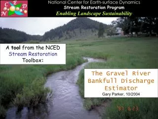
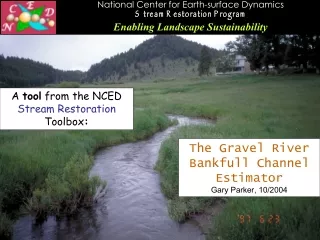
A tool from the NCED Stream Restoration Toolbox: The Gravel River Bankfull Channel Estimator Gary Parker, 10/2004
CAVEAT • This tool is provided free of charge. • Use this tool at your own risk. • In offering this tool, none of the following accept responsibility or liability for its use by third parties: • the National Center for Earth-surface Dynamics; • any of the universities and institutions associated with the National Center for Earth-surface dynamics; or • any of the authors of this tool.
The Gravel River Bankfull Channel Estimator This tool consists of a set of regression relations for predicting bankfull geometry of mobile-bed single-thread gravel bed streams in terms of bankfull discharge and bed surface median grain size. These relations can be used to a) help optimize the design of a restored channel to be as close as possible to its natural bankfull geometry, and b) help speed along the development toward this geometry by providing guidelines for preconstruction.
RIVERS ARE THE AUTHORS OF THEIR OWN GEOMETRY • Given enough time, rivers construct their own channels. • A river channel is characterized in terms of its bankfull geometry. • Bankfull geometryis defined in terms of river width and average depth at bankfull discharge. • Bankfull discharge is the flow discharge when the river is just about to spill onto its floodplain. • A river restoration scheme is likely to become more successful in a shorter amount of time if it takes into account the natural bankfull geometry of a channel. • This tool helps predict bankfull geometry for single-thread gravel- bed rivers with definable floodplains that actively move the gravel on their beds from time to time.
THIS TOOL IS FOR GRAVEL-BED STREAMS Little Wekiva River, Florida, USA: a sand-bed river. Raging River, Washington, USA: a gravel-bed river This tool addresses gravel-bed streams. Typical gravel-bed streams have bed surface median sizes Ds50 in the range from 8 to 256 mm. Boulder-bed streams have median sizes in excess of 256 mm. Sand-bed streams have median sizes between 0.062 and 2 mm.
THIS TOOL ADDRESSES SINGLE-THREAD RATHER THAN MULTIPLE-THREAD RIVERS Raging River, Washington, USA: a single-thread gravel-bed river Sunwapta River, Canada: a multiple-thread (braided) gravel-bed river This tool addresses single-thread streams. A single-thread stream has a single definable channel, although mid-channel bars may be present. A multiple-thread, or braided stream has several channels that intertwine back and forth.
THIS TOOL ADDRESSES MOBILE-BED RATHER THAN THRESHOLD CHANNELS Trinity Dam on the Trinity River, California, USA. A threshold channel forms immediately downstream. Raging River, Washington, USA: a mobile-bed river This tool addresses mobile-bed gravel streams. Such streams are competent to modify their beds because they mobilize all or nearly all gravel sizes on the bed from time to time during floods. Threshold channels are defined in the next slide.
THRESHOLD CHANNELS Threshold gravel-bed channels are channels which are barely not able to move the gravel on their beds, even during high flows. These channels form e.g. immediately downstream of dams, where their sediment supply is cut off. They also often form in urban settings, where paving and revetment have cut off the supply of sediment. Threshold channels are not the authors of their own geometry. The relations presented in this tool do not apply to them. Trinity Dam on the Trinity River, California, USA. A threshold channel forms immediately downstream.
PARAMETERS USED IN THIS TOOL • This tool uses the following parameters: • Bankfull discharge Qbf in cubic meters per second (m3/s) or cubic feet per second (ft3/s); • Bankfull channel width Bbf is meters (m) or feet (ft); • Bankfull cross-sectionally averaged channel depth Hbf in meters (m) or feet (ft); • Down-channel slope S (meters drop per meter distance or feet drop per feet distance). • Bed surface median grain size Ds50. This parameter is usually measured in millimeters (mm); the value must be converted to meters or feet in using the tool presented here. • These parameters are defined before the tool is introduced. If you are familiar with the parameters, click the hyperlink to jump to the tool.
BANKFULL PARAMETERS: THE RIVER AND ITS FLOODPLAIN floodplain A river constructs its own channel and floodplain. channel At bankfull flow the river is on the verge of spilling out onto its floodplain.
THE DEFINITION OF BANKFULL DISCHARGE Qbf Let denote river stage (water surface elevation in meters or feet relative to an arbitrary datum) and Q denote volume water discharge (cubic meters or feet per second). In the case of rivers with floodplains, tends to increase rapidly with increasing Q when all the flow is confined to the channel, but much less rapidly when the flow spills significantly onto the floodplain. The rollover in the curve defines bankfull discharge Qbf. The floodplain is often somewhat poorly-developed in mountain gravel-bed streams. Bankfull stage, however, can often still be determined by direct field inspection. Minnesota River and flooded floodplain, USA, during the record flood of 1965
CHARACTERIZING BANKFULL DISCHARGE Qbf • Bankfull discharge Qbf is used as a shorthand for the characteristic flow discharge that forms the channel. • One way to determine it is by means of direct measurement of the flow in a river. Since bankfull flow is not frequent, this method may be impractical in a river restoration scheme. • Another way to estimate it is from a stage-discharge curve, as described in the previous slide. In order to implement this, the river must be gaged near the reach of interest. • Another way is to estimate it using stream hydrology. It has been found that in gravel- bed streams bankfull flow is often reasonably estimated in terms of a peak flood discharge with a recurrence of 2 years (e.g. Williams, 1978 ). This corresponds to a flow discharge that has a 50% probability of occurring in any given year. • When none of the above methods can be implemented, Qbf can be estimated from bankfull channel characteristics using the tool BankfullDischargePredictor.ppt of this toolbox.
CHARACTERIZING BANKFULL CHANNEL GEOMETRY: BANKFULL WIDTH Bbf AND BANKFULL DEPTH Hbf Bankfull geometry is here defined in terms of the average characteristics of a channel cross-section at bankfull stage, i.e. when the flow is at bankfull discharge. Here the key parameters are: bankfull width Bbf and cross-sectionally averagedbankfull depthHbf. These parameters should be determined from averages of values determined at several cross-sections along the river reach of interest.
CAVEAT: NOT ALL RIVERS HAVE A DEFINABLE BANKFULL GEOMETRY! Rivers in bedrock often have no active floodplain, and thus no definable bankfull geometry. Wilson Creek, Kentucky: a bedrock stream. Image courtesy A. Parola. Highly disturbed alluvial rivers are often undergoing rapid downcutting. What used to be the floodplain becomes a terrace that is almost never flooded. Time is required for the river to construct a new equilibrium channel and floodplain. Reach of the East Prairie Creek, Alberta, Canada undergoing rapid downcutting due to stream straightening. Image courtesy D. Andres. The relations presented in this tool do not apply to bedrock streams, or disturbed alluvial streams with no active floodplain. They may, however, be used to estimate characteristics of the ultimate equilibrium alluvial channel that will evolve in time.
FIELD MEASUREMENT OF BANKFULL CHANNEL GEOMETRY Not all field channels have definable bankfull geometries. Even when a channel does have a definable bankfull geometry, some experience and judgement is required to measure it. In the future a worked example complete with photographs and data files will be added to the toolbox. Until this is done, the user is urged to spend some time to determine how bankfull geometry should be determined.
CHARACTERIZING BED SEDIMENT IN GRAVEL-BED STREAMS: MEDIAN SURFACE SIZE Ds50 Armored surface Gravel-bed streams usually show a surface armor. That is, the surface layer is coarser than the substrate below. substrate Bed sediment of the River Wharfe, U.K., showing a pronounced surface armor. Photo courtesy D. Powell.
SURFACE AND SUBSTRATE MEDIAN SIZES Here the surface median size is denoted as Ds50 and the substrate median size is denoted as Dsub50. The surface is said to be armored when Ds50/Dsub50 > 1. This ratio also provides a rough estimate of ability of the stream to move its own gravel. Low values of Ds50/Dsub50 (e.g. < 1.3, i.e. relatively weak armoring) are generally indicative of relatively high mean annual sediment transport rates, whereas high values of Ds50/Dsub50 (e.g. > 4, relatively strong armor) are generally indicative of relatively low mean annual sediment transport rates (Dietrich et al., 1989). Notes on bed sampling, grain size distributions and the determination of median sediment size are given in and Appendix (slides 35-41) toward the end of this presentation. To jump to them click the hyperlink bed sampling.
CHARACTERIZING DOWN-CHANNEL SLOPE S Down-channel bed slope should be determined from a survey of the long profile of the channel centerline. The reach chosen to determine bed slope should be long enough to average over any bars and bends in the channel, which are associated with local elevation highs and lows.
CHANNEL SLOPE VERSUS VALLEY SLOPE In the figure to the left, down-channel bed slope S is the difference in bed elevation from A to B divided by the along-channel distance from A to B (red line). Down-valley bed slope Sv is the difference in elevation from A to B divided by the along-valley distance from A to B (blue line). The ratio between the down-channel distance from A to B and the down-valley distance from A to B is known as channel sinuosity . For a channel that is parallel to the valley (essentially straight) = 1. Gravel-bed rivers tend to have sinuosities ranging from about 1.2 to 1.8, with lower values generally at higher slopes. The relation between downchannel slope S and down-valley slope Sv is given as
SINGLE-THREAD GRAVEL-BED RIVERS HAVE CONSISTENT BANKFULL GEOMETRIES! • This is illustrated here using data from four sources: • 16 streams flowing from the Rocky Mountains in Alberta, Canada (Kellerhals et al., 1972); • 23 mountain streams in Idaho (Parker et al., 2003); • 23 upland streams in Britain (mostly Wales) (Charlton et al. 1978); • 10 reaches along the upper Colorado River, Colorado (Pitlick and Cress, 2002) (Each reach represents an average of several subreaches.) • The original data for Qbf, Bbf, Hbf, S and Ds50 for each reach can be found in the companion Excel file, ToolboxGravelBankfullData.xls.
RANGE OF PARAMETERS Among all four sets of data, the range of parameters is as given below: Bankfull discharge Qbf (in meters3/sec) 2.7 ~ 5440 Bankfull width Bbf (in meters) 5.24 ~ 280 Bankfull depth Hbf (in meters) 0.25 ~ 6.95 Channel slope S 0.00034 ~ 0.031 Surface median size Ds50 (in mm) 27 ~ 167 These ranges approximate the range of applicability of the relations presented in this tool.
DIMENSIONLESS PARAMETERS The universality of bankfull characteristics of single-thread gravel-bed rivers is expressed with the use of dimensionless parameters. Dimensionless bankfull depth, width and discharge are defined as where g denotes the acceleration of gravity. These parameters can be computed in either SI or English. When using SI units, Hbf, Bbf and Ds50 should be in meters (convert Ds50 from mm), Qbf should be in cubic meters per second, and g should take a value of 9.81 meters/sec2. When using English units, Hbf, Bbf and Ds50 should be in feet (convert Ds50 from mm), Qbf should be in cubic feet per second, and g should take a value of 32.2 ft/sec2. Note that down-channel bed slope S is already dimensionless (meter drop per meter distance or feet drop per feet distance).
WHAT THE DATA SAY The four data sets tell a consistent story of bankfull channel characteristics. Dimensionless width Dimensionless depth Down-channel bed slope
REGRESSION RELATIONS FOR BANKFULL CHANNEL CHARACTERISTICS To a high degree of approximation, S
WHY DOES THE RELATION FOR SLOPE SHOW THE MOST SCATTER? • Rivers can readjust their bankfull depths and widths over short geomorphic time, e.g. hundreds to thousands of years. • Readjusting river valley slope involves moving large amounts of sediment over long reaches, and typically requires long geomorphic time (tens of thousands of years or more). • As a result, valley slope can often be considered to be an imposed parameter that the river is not free to adjust in short geomorphic time. This concept should be used in most river restoration projects. • Varying the channel sinuosity allows for some variation in channel slope S at the same valley slope Sv.
THE TOOL CONSISTS OF THREE RELATIONS Caution: use these relations subject to the caveats of Slides 5, 6, 7, 8 and 14!
TOOL IMPLEMENTATION: BANKFULL GEOMETRY PREDICTED FROM THE REGRESSION RELATIONS Stop the slide show and double-click to activate the Excel spreadsheet. The spreadsheet is then live: you can change input as you please. Caution: use the relations subject to the caveats of Slides 5, 6, 7, 8 and 14!
A WORKED EXAMPLE OF RIVER RESTORATION A reach of river had the following characteristics before intervention. Qbf = 600 m3/s (2-year flood) Bbf = 96 m Hbf = 2.9 m S = 0.00015 Ds50 = 46 mm A dam was constructed on the reach. As a result all flood flows were cut off, and the channel was turned into a threshold channel. As part of a river restoration scheme, annual flooding is to be restored using controlled reservoir releases. No gravel is to be fed in immediately downstream of the dam, so that reach will remain a threshold channel. Gravel of similar size to that which prevailed in the channel enters the stream at the first major tributary. The effective 2-year recurrence flood of the restoration scheme is 220 m3/s. Compute the bankfull characteristics of the restored mobile-bed channel downstream of the first tributary. Caution: use the relations subject to the caveats of Slides 5, 6, 7, 8 and 14!
WORKED EXAMPLE contd. In this example, the original bankfull discharge was 600 m3/s. The intervention of a dam cut off all flood flows. The restoration scheme brings back a 2-year flood of 220 m3/s. Using this value as the new bankfull discharge, it is apparent that the channel must shrink to fit it. That is, both bankfull width Bbf and bankfull depth Hbf must reduce over time to fit the reduced bankfull discharge. In nature, this is accomplished by means of sediment deposition, augmented by vegetal encroachment. In time, a smaller but morphologically (and presumably ecologically) healthy channel should evolve. This natural process may take decades or centuries. A river restoration scheme can speed the evolution to this new state by partially pre-installing the new channel. Caution: use the relations subject to the caveats of Slides 5, 6, 7, 8 and 14!
CALCULATIONS FOR THE ORIGINAL CHANNEL Stop the slide show and double-click to activate the Excel spreadsheet. The spreadsheet is then live: you can change input as you please. Caution: use the relations subject to the caveats of Slides 5, 6, 7, 8 and 14!
COMPARISON BETWEEN THE OBSERVED ORIGINAL CHANNEL AND THAT COMPUTED FROM THE REGRESSION RELATIONS The values predicted from the regression relations are similar to the observed values, at least within the scatter of the data used to determine them. Caution: use the relations subject to the caveats of Slides 5, 6, 7, 8 and 14!
CALCULATIONS FOR RESTORATION SCHEME Double-click to activate the Excel spreadsheet. The spreadsheet is live: you can change input as you please. Caution: use the relations subject to the caveats of Slides 5, 6, 7, 8 and 14!
BANKFULL CHARACTERISTICS OF THE RESTORED CHANNEL Caution: use the relations subject to the caveats of Slides 5, 6, 7, 8 and 14!
BANKFULL CHARACTERISTICS OF THE RESTORED CHANNEL contd. The restored bankfull channel should have 63% of the original width and 68% of the original depth. These percentages should be applied to the values for the original channel (rather than those predicted from the regression relations) if they are known. It may take decades or centuries for the new channel to evolve on its own; channel modification can help speed the evolution to the new dimensions by providing a head start. Caution: use the relations subject to the caveats of Slides 5, 6, 7, 8 and 14!
SINUOSITY OF THE RESTORED CHANNEL Valley slope Sv is assumed to be constant. As a result, the relation between sinuosity and slope is where the subscripts “o” and “ar” denote “original” and “after restoration.” The numbers in the above table give: Thus the restored channel should be somewhat less sinuous than the original channel before intervention.
FURTHER CAVEATS • It is not possible to restore a stream in a meaningful way by supplying it with a discharge that is constant the year round. Channel and floodplain formation, cleaning of the gravel bed and renewal of the riparian ecosystem all require both flood and low flows. • A restored flood regimen should not consist of only a very brief spike. The restored flood hydrograph should have a duration that is at least somewhat similar to the original one before intervention. If the flood hydrograph is too short it will be insufficient to a) overturn the gravel and b) rip out excessive encroaching vegetation. • The flood regimen should not be restored without a gravel supply. If the gravel supply of the first major tributary downstream of a dam is insufficient, or too fine, it may be necessary to feed gravel in addition to restoring flood flows. A threshold channel will develop or be maintained on any reach that has no gravel supply.
APPENDIX: SEDIMENT SIZE DISTRIBUTIONS IN GRAVEL-BED STREAMS Armored surface Implementation of the regression relations requires a knowledge of the median size of the surface armor Ds50. This value must be determined by sampling the bed. In order to characterize the bed sediment of the stream the surface and substrate should be sampled separately. The results of sampling are plotted in terms of percent finer versus grain size (mm) as illustrated below. substrate Bed sediment of the River Wharfe, U.K., showing a pronounced surface armor. Photo courtesy D. Powell.
WOLMAN COUNT OF SURFACE SEDIMENT The simplest way to sample a gravel bed surface is by means of a Wolman count (Wolman, 1954). The gravel surface is paced, and at set intervals a particle next to the toe of one’s foot is sampled. The sampling should be chosen so as to capture the spatial variation in bed texture. Grain size is characterized in terms of the b-axis of a grain (middle axis as measured with a caliper) or the size of the smallest square through which the grain will fit. A series grain size ranges is set for estimating the grain size distribution. In analyzing a Wolman sample, it is necessary to determine the number of grains in each range. These numbers are used to determine the grain size distribution. A sample calculation is given in the live spreadsheet of the next slide. Wolman sampling is not practical for sand-sized or smaller grains. More specifically, grains finer than about 4 mm should not be included in a sample. It should be understood that this method misses the finer grains in the surface.
GRAIN SIZE DISTRIBUTION FROM WOLMAN COUNT The live spreadsheet to the right shows a worked example for a Wolman count. Stop the slide show and double-click to activate it. It is customary to plot grain size on a logarithmic scale when presenting grain size distributions.
KLINGEMAN SAMPLE OF SURFACE SEDIMENT The methodology for a Klingeman sample of the surface sediment is outlined in Klingeman et al. (1979). A circular patch of sediment is specified on the bed. The largest grain that shows any exposure on the bed surface is located and removed. All of the bed material (including sand) is then sampled down to the level of the bottom of the hole created by removing the largest grain. The resulting sample is analyzed by mass (weight) rather than number. A Klingeman sample captures the sand as well as the gravel in the surface layer. Sampling is, however, more laborious than that required for a Wolman sample. In addition, several Klingeman samples at different locations may be needed to characterize the spatial variability of the surface sediment. A sample calculation is given in the live spreadsheet of the next page.
KLINGEMAN SAMPLE OF SURFACE SEDIMENT contd. The live spreadsheet to the right shows a worked example for a Klingeman sample. Stop the slide show and double-click to activate it.
BULK SAMPLE OF SUBSTRATE The substrate may be sampled in bulk. The surface layer is first carefully stripped off down to the depth of the bottom of the largest particle exposed on the surface. A bulk sample (e.g. cubical) volume of substrate is then excavated. According to the guidelines of Church et al. (1987), the mass (weight) of the sample should be at least 100 times the mass (weight) of the largest grain contained in the sample. Several such samples may be needed to characterize the spatial variability of the substrate. The sample is analyzed in terms of mass (weight) rather than number.
MEDIAN SIZE It is useful to characterize a sample in terms of its median size D50, i.e. the size for which 50% of the material is finer. To do this, find the grain sizes D1 and D2 such that the percentage content F1 is the highest value below 50% and the percentage content F2 is the lowest percentage above 50%. The median size D50 is then estimated by log-linear interpolation as: For example, in the Klingeman sample of slide 13: D1 = 32 mm, F1 = 45.24%, D2 = 64 mm and F2 = 59.52%. The calculation of D50 is illustrated in terms of the live spreadsheet below. Stop the slide show and double-click to activate it.
REFERENCES Charlton, F. G., Brown, P. M. and R. W. Benson 1978 The hydraulic geometry of some gravel rivers in Britain. Report INT 180, Hydraulics Research Station, Wallingford, England, 48 p. Church, M. A., D. G. McLean and J. F. Wolcott 1987 River bed gravels: sampling and analysis. In Sediment Transport in Gravel-bed Rivers, Thorne, C. R., J. C. Bathurst, and R. D. Hey, eds., John Wiley & Sons, 43-79. Dietrich, W. E., J. W. Kirchner, H. Ikeda and F. Iseya 1989 Sediment supply and the development of the coarse surface layer in gravel-bedded rivers. Nature, 340, 215-217. Ferguson, R. I. 1987 Hydraulic and sedimentary controls of channel pattern. In Rivers: Environment and Process, K. Richards. ed., Blackwell, Oxford, 129-158. Kellerhals, R., Neill, C. R. and D. I. Bray 1972 Hydraulic and geomorphic characteristics of rivers in Alberta. River Engineering and Surface Hydrology Report, Research Council of Alberta, Canada, No. 72-1.
REFERENCES contd. Klingeman, P. C., C. J. Chaquette, and S. B. Hammond 1979 Bed Material Characteristics near Oak Creek Sediment Transport Research Facilities, 1978-1979. Oak Creek Sediment Transport Report No. BM3, Water Resources Research Institute, Oregon State University, Corvallis, Oregon, June. Parker, G., Toro-Escobar, C. M., Ramey, M. and S. Beck 2003 The effect of floodwater extraction on the morphology of mountain streams. Journal of Hydraulic Engineering, 129(11). Parker, G. 2004 Quasi-universal relations for bankfull hydraulic geometry of single- thread gravel-bed rivers . In preparation. Pitlick, J. and R. Cress 2002 Downstream changes in the channel of a large gravel bed river. Water Resources Research38(10), 1216, doi:10.1029/2001WR000898, 2002. Williams, G. P. 1978 Bankfull discharge of rivers. Water Resources Research, 14, 1141-1154. Wolman, M.G. 1954. A method of sampling coarse river bed material. Trans. Am. Geophys. Union, 35, 951–956.