Download
1 / 30
330 likes | 794 Views
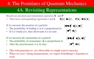
4. The Postulates of Quantum Mechanics. 4A. Revisiting Representations. Recall our position and momentum operators R and P They have corresponding eigenstate r and k If we measure the position of a particle: The probability of finding it at r is proportional to

E N D
4. The Postulates of Quantum Mechanics 4A. Revisiting Representations Recall our position and momentum operators R and P • They have corresponding eigenstater and k If we measure the position of a particle: • The probability of finding it at r is proportional to • If it is found at r, then afterwards it is in state If we measure the momentum of a particle: • The probability of momentum k is proportional to • After the measurement, it is in state • This will generalize to any observable we might want to measure • When we aren’t doing measurements, we expect Schrödinger’s Equation to work
4B. The Postulates Vector Space and Schrödinger’s Equation Postulate 1: The state vector of a quantum mechanical system at time t can be described as a normalized ket |(t) in a complex vector space with positive definite inner product • Positive definite just means • At the moment, we don’t know what this space is Postulate 2: When you do not perform a measurement, the state vector evolves according to where H(t) is an observable. • Recall that observable implies Hermitian • H(t) is called the Hamiltonian
The Results of Measurement Postulate 3: For any quantity that one might measure, there is a corresponding observable A, and the results of the measurement can only be one of the eigenvalues a of A • All measurements correspond to Hermitian operators • The eigenstates of those operators can be used as a basis Postulate 4: Let {|a,n} be a complete orthonormal basis of the observable A, with A|a,n = a|a,n, and let |(t) be the state vector at time t. Then the probability of getting the result a at time t will be • This is like saying the probability it is at r is proportional to |(r)|2
The State Vector After You Measure Postulate 5: If the results of a measurement of the observable A at time t yields the result a, the state vector immediately afterwards will be given by • The measurement is assumed to take zero time THESE ARE THE FIVE POSTULATES • We haven’t specified the Hamiltonian yet • The goal is not to show how to derive the Hamiltonian from classical physics, but to find a Hamiltonian that matches our world
Comments on the Postulates • I have presented the Schrödinger picture with state vector postulates with the Copenhagen interpretation • Other authors might list or number them differently • There are other, equally valid ways of stating equivalent postulates • Heisenberg picture • Interaction picture • State operator vs. state vector • Even so, we almost always agree on how to calculate things • There are also deep philosophical differences in some of the postulates • More on this in chapter 11
Continuous Eigenvalues • The postulates as stated assume discrete eigenstates • It is possible for one or more of theselabelsto be continuous • If the residual labels are continuous, just replace sums by integrals • If the eigenvalue label is continuous, the probability of getting exactly will be zero • We need to give probabilities that lies in some range, 1 < < 2. • We can formally ignore this problem • After all, all actual measurements are to finite precision • As such, actual measurements are effectively discrete (binning)
Modified Postulates for Continuous States Postulate 4b: Let {|,} be a complete orthonmormal basis of the observable A, with A|, = |,, and let |(t) be the state vector at time t. Then the probability of getting the result between 1 and 2 at time t will be Postulate 5b: If the results of a measurement of the observ-able A at time t yields the result in the range 1 < < 2, the state vector immediately afterwards will be given by
4C. Consistency of the Postulates Consistency of Postulates 1 and 2 • Postulate 1 said the state vector is always normalized; postulate 2 describes how it changes • Is the normalization preserved? • Take Hermitian conjugate • Mulitply on left and right to make these: • Subtract:
Consistency of Postulates 1 and 5 • Postulate 1 said the state vector is always normalized; postulate 5 des-cribes how it changes when measured • Is the normalization preserved?
Probabilities Sum to 1? • Probabilities must be positive and sum to 1 Postulate 4 Independent of Basis Choice? • Yes Postulate 5 Independent of Basis Choice? • Yes
Sample Problem A system is initially in the state When S2 is measured, (a) What are the possible outcomes and corresponding probabilities, (b) For each outcome in part (a), what would be the final state vector? • We need eigenvalues and eigenvectors
Sample Problem (2) (b) For each outcome in part (a), what would be the final state vector? • If 0: • If 22:
Comments on State Afterwards: • The final state is automatically normalized • The final state is always in an eigenstate of the observable, with the measured eigenvalue • If you measure it again, you will get the same value and the state will not change • When there is only one eigenstate with a given eigenvalue, it must be that eigenvector exactly • Up to an irrelevant phase factor
4D.Measurement and Reduction of State Vector How Measurement Changes Things Whenever you are in an eigenstate of A, and you measure A, the results are certain, and the measurement doesn’t change the state vector • Eigenstates with different eigenvalues are orthogonal • The probability of getting result a is then • The state vector afterwards will be: • Corollary: If you measure something twice, you get the same result twice, and the state vector doesn’t change the second time
Sample Problem • We need eigenvalues and eigenvectors for both operators • Eigenvalues for both are ½ A single spin ½ particle is described by a two-dimensional vector space. Define the operators The system starts in the state If we successively measure Sz, Sz, Sx, Sz, what are the possible outcomes and probabilities, and the final state? • It starts in an eigenstate of Sz • So you get + ½ , and eigenvector doesn’t change 100% 100%
Sample Problem (2) If we successively measure Sz, Sz, Sx, Sz, what are the possible outcomes and probabilities, and the final state? • When you measure Sx next, we find that the probabilities are: • Now when you measure Sz, the probabilities are: 50% 50% 50% 50% 50% 50%
Commuting vs. Non-Commuting Observables • The first two measurements of Sz changed nothing • It was still in an eigenstate of Sz • But when we measured Sx, it changed the state • Subsequent measurement of Szthen gave a different result The order in which you perform measurements matters • This happens when operators don’t commute, AB BA • If AB = BA then the order you measure doesn’t matter • Order matters when order matters Complete Sets of Commuting Observables (CSCO’s) • You can measure all of them in any order • The measurements identify | uniquely up to an irrelevant phase
4E. Expectation Values and Uncertainties Expectation values • If you measure Aand get possible eigenvalues {a}, the expectation value is • There is a simpler formula: • Recall: • The old way of calculating expectation value of p: • The new way of calculating expectation value of p:
Uncertainties • In general, the uncertainty in a measurement is the root-mean-squared difference between the measured value and the average value • There is a slightly easier way to calculate this, usually:
Generalized Uncertainty Principle • We previously claimed and we will now prove it • Let A and B be any two observables • Consider the following mess: • The norm of any vector is positive: • The expectation values are numbers, they commute with everything • Now substitute • This is two true statements, the stronger one says:
Example of Uncertainty Principle • Let’s apply this to a position and momentum operator • This provides no useful information unless i = j. Sample Problem Get three uncertainty relations involving the angular momentum operators L
4F. Evolution of Expectation Values General Expression • How does A change with time due to Schrödinger’s Equation? • Take Hermitian conj. of Schrödinger. • The expectation value will change • In particular, if the Hamiltonian doesn’t depend explicitly on time:
Ehrenfest’s Theorem: Position Suppose the Hamiltonian is given by How do P and R change with time? • Let’s do X first: • Now generalize:
Ehrenfest’s Theorem: Momentum • Let’s do Px now: • Generalize Interpretation: • Revolution: v = p/m • Pevolution: F = dp/dt
Sample Problem The 1D Harmonic Oscillator has Hamiltonian Calculate X and P as functions of time • We need 1D versions of these: • Combine these: • Solve it: • A and B determined by initial conditions:
4G. Time Independent Schrödinger Equation Finding Solutions • Before we found solution when H was independent of time • We did it by guessing solutions with separation of variables: • Left side is proportional to |, right side is independent of time • Both sides must be a constant times | • Time Equation is not hard to solve • It remains only to solve the time-independent Schrödinger Equation
Solving Schrödinger in General Given |(0), solve Schrödinger’s equation to get |(t) • Find a complete set of orthonormal eigenstates of H: • Easier said than done • This will be much of our work this year • These states are orthonormal • Most general solution to time-independent Schrödinger equation is • The coefficients cn can then be found using orthonormality:
Sample Problem An infinite 1D square well with allowed region 0 < x < a has initial wave function in the allowed region. What is (x,t)? • First find eigenstates and eigenvalues • Next, find the overlap constants cn • sin(½n) = 1, 0, -1, 0, 1, 0, -1, 0, …
Sample Problem (2) An infinite 1D square well with allowed region 0 < x < a has initial wave function in the allowed region. What is (x,t)? • Now, put it all together
Irrelevance of Absolute Energy In 1D, adding a constant to the energy makes no difference • Are these two Hamiltonians equivalent in quantum mechanics? • These two Hamiltonians have the same eigenstates • The solutions of Schrödinger’s equation are closely related • The solutions are identical except for an irrelevant phase