Download
1 / 40
540 likes | 1.24k Views
Basic Concepts of Economics. Use basic economic concepts to explain changes in natural resource base and environmental quality. Prepared by Husam Al-Najar. Content. What is economics? Basics of microeconomics Three basic theories Rational behavior Opportunity costs Marginal analysis

E N D
Basic Concepts of Economics Use basic economic concepts to explain changes in natural resource base and environmental quality Prepared by Husam Al-Najar
Content • What is economics? • Basics of microeconomics • Three basic theories • Rational behavior • Opportunity costs • Marginal analysis • Making choices • Supply & demand model • Cost estimation methods
Definitions • Economics: A social science that studies and influences human behavior • Microeconomics studies how individuals use limited resources to meet various needs and consequences of their decisions • Macroeconomics studies the determinants of aggregate level of economic activities
Basics of Microeconomics A fundamental contradiction in life: • Resources are limited or scarce • Human wants are unlimited or insatiable Therefore, choices must be made! Economics is about making choices!
Theory 1: Rational Behavior • People know what they want; • Their behaviors are consistent with what they want; • Assume information is given.
Opportunity Cost • The cost of anything in terms of other things given up or sacrificed. • What would you be doing right now if you did not come to this lecture? • “No pain, no gain” • “There is no such a thing as free lunch!”
Marginal Analysis • Effects of per unit change in activity • effects of converting another 100 ha of forests • effects of consuming another 100 liter of water • effects of catching another 100 tons of fish • effects of reducing another 100 tons of pollutants • The effects have two sides: benefits & costs
Diminishing Marginal Benefits • As you increase your activity while other things remain constant, the benefits from each additional unit of your activity declines. • The benefits of eating the 2nd, 3rd, and 4th pizza?
Increasing Marginal Costs • As you increase your activity while other things remain constant, the costs of carrying out each additional unit of your activity increases. • Costs of attending to the 2nd, 3rd, and 4th week of the lecture?
Making Choices How to do? choose the least cost combination of capital, land, labor, and technology
Law of Supply • The quantity supplied will increase if the price does up, holding other things constant. • This relationship reflects increasing marginal cost of supply (MC) • Determinants of supply: factors other than price that influence supply: number of producers, cost of production, and technology
Law of Demand • Demand will increase if the price goes down, holding other things constant. • This relationship reflects diminishing marginal benefit from consumption • Determinants of demand: factors other than price that influence demand: income, number of consumers, and preferences
Supply and Demand Modelin a perfectly competitive market Price Supply = MC P’ Demand = MB Q’ Quantity
Individual Producerin a perfectly competitive market Price Supply = MC P’ Demand = MB Quantity Q’
Cost Behavior Fixed Cost Behavior Variable Cost Behavior £ £ Relevant Range Activity Activity
The Behavior of a Mixed Cost Linearity Assumption Total Costs £Cost Fixed Costs Variable Costs Number of Units Produced Y = F + VX
Step-Variable Costs Linearity Assumption £Cost Narrow Width Number of Units Produced
Step-Fixed Costs Linearity Assumption £Cost Wider Width Number of Units Produced
Cost Estimation Method • Used by managers to predict/plan costs at various activity levels • Useful when cost information is not broken into fixed and variable components • Five common methods • Engineering method • Account analysis • Scattergraph • High-Low • The Method of least squares (Regression)
The Goal of Estimation • Goal = create a cost equation • TC = FC + VCx • TC = total costs • FC = fixed costs • VC = slope of line (variable costs) • x = units produced/sold
1. Engineering Method • This method is based on the use of engineering analyses of technological relationships between inputs and outputs – for example, methods study, work sampling and time and motion studies. • The approach is appropriate when there fiscal relationship between costs and the cost driver. • The procedure when under-taking an engineering study is to make an analysis based on direct observations of the underlying physical quantities required for an activity and then to convert the final results into cost estimates. • Engineers, who are familiar with the technical requirements, estimate the quantities of materials and the labour and machine hours required for various operations; prices and rates are then applied to the physical measures to obtain the cost estimates. • The Engineering method is useful for estimating costs of repetitive processes where input-output relationships are clearly defined.
Used to estimating fixed and variable costs Step 1: Classify costs as variable or fixed Requires professional judgment Step 2: Determine variable costs per unit Total Variable Costs Activity Level 2. Account Analysis • Step 3:Determine fixed costs • Add all fixed costs together The function is the total of variable and fixed costs TC = VCx + FC
Used to estimate fixed and variable costs to determine how costs and activity levels change Step 1: Acquire cost information over several periods Step 2: Graph the data Step3 : Eyeball a linear relationship 3. Scatter graph Approach
Nonlinear Relationship * * Total production cost * * * 0 Unit produced
Upward Shift in Cost Relationship * * * * Total production cost * * 0 Unit produced
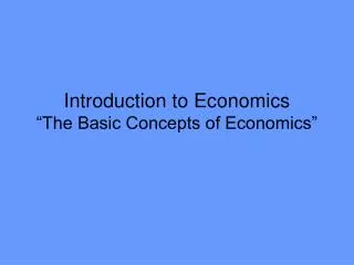
Presence of Outliers * * * * Total production cost * * 0 Unit produced
Results: Variable cost = Line slope Fixed costs = Y-intercept 4. High-Low Method • Used to estimating fixed and variable costs at various levels of activity • Uses two data points, the high and low levels of activity and their related total overhead costs
Select high and low ‘activity’ levels first, then corresponding costs. Key Point: High-Low Method Step 1: Select the high and low data activity points. Step 2: Subtract the smallest from the largest cost and the smallest from the largest activity and use the changes in the following formula. Change in Cost = Variable cost per unit Change in volume
High-Low Method Step 3: Pick one point: Substitute the total cost of one of the points for “y” in the equation: y = mx + b Step 4: Substitute the variable cost from step 2 into the formula for “m” Slope Step 5: Substitute the number of activity units for the data point chosen for “x”
High-Low Method Continued Step 6: Solve for fixed costs “b” Step 7: Determine the cost formula to use in estimating the mixed costs at various levels in the following format: y= m x + b Only two letter variables will be displayed in the formula–X and Y. The other letters—m and b should be replaced by the respective amounts.
Example: High-Low Method Month Utility Costs Units Produced January £2,000 200 February 2,500 400 March 4,500 600 April 5,000 800 May 7,500 1,000
The High-Low Method (continued) Y = F + VX Variable Cost Rate (V) = (Y2 - Y1)/(X2 - X1) V = (£7,500-£2,000)/(1,000-200) V = £5,500/800 V = £6.875 per unit Y = F + VX £7,500 = F + £6.875 (1,000) F = £7,500 - £6,875 F = £625 The cost formula using the high-low method is: Y = £625 + £6.875 (X)
5. The Least –Squares Method • The method determines mathematically the regression line of best fit. It is based on the principle that the sum of the squares of the vertical deviations from the line that is established using the method is less than the sum of the squares of the vertical deviations from any other line that might be drawn. The regression equation for a straight line that meets this requirement can be found from the following two equations by solving for a and b. • Ey=Na+bEx………..(1) • Exy=aEx +bex2……(2) • Where N is the number of observations.
Example: The Least Square • Hours x Maintenance Cost y • 90 1500 • 150 1950 • 60 900 • 30 900 • 180 2700 • 150 2250 • 120 1950 • 180 2100 • 90 1350 • 30 1050 • 120 1800 • 60 1350
Solution to the Problem • Hours x Maintenance Cost y X2 xy • 90 1500 8100 135,000 • 150 1950 22500 292,500 • 60 900 3600 54,000 • 30 900 900 27,000 • 180 2700 32,400 486,000 • 150 2250 22500 337500 • 120 1950 14400 234000 • 180 2100 32400 378000 • 90 1350 8100 121500 • 30 1050 900 31500 • 120 1800 14400 216000 • 60 1350 360081000 • Ex = 1260Ey = 19800Ex2 = 163800Exy = 2394000
Solution (Continued) • Using Normal Equation, we have: • 19800 = 12a + 1260b…………Equation (1). • 2394000 = 1260a + 163800b…..Equation (2). • To solve for b, multiply equation (1) by 105 (1260/12), to give: • 2079000 = 1260a + 132300b……Equation (3) • Subtracting equation (3) from equation (2), the ‘a’ terms will cancel out to yield 315000 = 31500b. Therefore, b = £10. • Substituting this value of b into equation (1) and solving for a, we have • 19800 = 12a + 1260 x 10 • As a result, a = 600. • Substituting this values of a and b into regression equation y = a + bx, we find that the regression line (i.e. cost function can be described by • Y = £600 + £10x. • We can now use this formula to predict the cost incurred at different activity levels, including those for which we have no past observations.