Previous Lecture: Motifs

1. Previous Lecture: Motifs

2. This Lecture Introduction to Biostatistics and Bioinformatics Phylogenetics

3. Learning Objectives • Molecular Evolution • Calculating Distances • Clustering Algorithms • CladisticMethods • Computer Software

4. Evolution • The theory of evolution is the foundation upon which all of modern biology is built. • From anatomy to behavior to genomics, the scientific method requires an appreciation of changes in organisms over time. • It is impossible to evaluate relationships among gene sequences without taking into consideration the way these sequences have been modified over time

5. Nothing in biology makes sense except in the light of evolution. • Theodosius Dobzhansky, 1973

6. Relationships Similarity searches and multiple alignments of sequences naturally lead to the question: “How are these sequences related?” and more generally: “How are the organisms from which these sequences come related?”

8. The purpose of a phylogenetic tree is to illustrate how a group of objects (usually genes or organisms) are related to one another

9. Taxonomy • The study of the relationships between groups of organisms is called taxonomy, an ancient and venerable branch of classical biology. • Taxonomy is the art of classifying things into groups — a quintessential human behavior — established as a mainstream scientific field by Carolus Linnaeus (1707-1778).

11. Phylogenetics • Evolutionary theory states that groups of similar organisms are descended from a common ancestor. • Phylogenetic systematics (cladistics) is a method of taxonomic classification based on their evolutionary history. • It was developed by Willi Hennig, a German entomologist, in 1950.

12. Cladistics and Phenetics • Cladistic approach: Trees are drawn based on the conserved characters • Phenetic approach: Trees are based on some measure of distance between the leaves • Molecular phylogenies are inferred from molecular (usually sequence) data • either cladistic (e.g. gene order) or phenetic

13. Cladistic Methods • Evolutionary relationships are documented by creating a branching structure, termed a phylogeny or tree, that illustrates the relationships between the sequences. • Cladistic methods construct a tree (cladogram) by considering the various possible pathways of evolution and choose from among these the best possible tree. • A phylogram is a tree with branches that are proportional to evolutionary distances.

15. Classes of algorithm used to infer phylogeny from sequence • Distance methods • Parsimony • Likelihood • Probabilistic methods

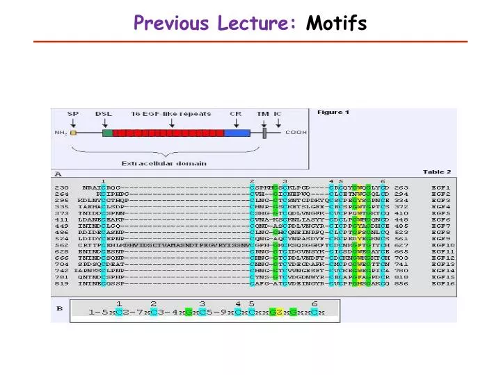
16. Molecular Evolution • Phylogenetics often makes use of numerical data, (numerical taxonomy) which can be scores for various “character states” such as the size of a visible structure or it can be DNA sequences. • Similarities and differences between organisms can be coded as a set of characters, each with two or more alternative character states. • In an alignment of DNA sequences, each position is a separate character, with four possible character states, the four nucleotides.

17. DNA is a good tool for taxonomy DNA sequences have many advantages over classical types of taxonomic characters: • Character states can be scored unambiguously • Large numbers of characters can be scored for each individual • Information on both the extent and the nature of divergence between sequences is available (nucleotide substitutions, insertion/deletions, or genome rearrangements)

18. Aaat tcg ctt cta gga atc tgc cta atc ctg B ... ..a ..g ..a .t. ... ... t.. ... ..a C ... ..a ..c ..c ... ..t ... ... ... t.a D ... ..a ..a ..g ..g ..t ... t.t ..tt.. Each nucleotide difference is a character

19. Sequences Reflect Relationships • After working with sequences for a while, one develops an intuitive understanding that for a given gene, closely related organisms have similar sequences and more distantly related organisms have more dissimilar sequences. These differences can be quantified. • Given a set of gene sequences, it should be possible to reconstruct the evolutionary relationships among genes and among organisms.

21. What Sequences to Study? • Different sequences accumulate changes at different rates - chose level of variation that is appropriate to the group of organisms being studied. • Proteins (or protein coding DNAs) are constrained by natural selection - better for very distant relationships • Some sequences are highly variable (rRNA spacer regions, immunoglobulin genes), while others are highly conserved (actin, rRNA coding regions) • Different regions within a single gene can evolve at different rates (conserved vs. variable domains)

22. Orthologs vs. Paralogs • When comparing gene sequences, it is important to distinguish between identical vs. merely similar genes in different organisms. • Orthologs are homologous genes in different species with analogous functions. • Paralogs are similar genes that are the result of a gene duplication. • A phylogeny that includes both orthologs and paralogs is likely to be incorrect. • Sometimes phylogenetic analysis is the best way to determine if a new gene is an ortholog or paralog to other known genes.

23. Ancestral gene A (globin) Duplication A B (myoglobin) (hemoglobin) Speciation A1 B1 A2 B2 (mouse) (human)

24. Disclaimers Before describing any theoretical or practical aspects of phylogenetics, it is necessary to give some disclaimers. This area of computational biology is an intellectual minefield! • Neither the theory nor the practical applications of any algorithms are universally accepted throughout the scientific community. • The application of different software packages to a data set is very likely to give different answers; minor changes to a data set are also likely to profoundly change the result.

26. A modern revision of the seals and sea lions

27. Genes vs. Species • Relationships calculated from sequence data represent the relationships between genes, this is not necessarily the same as relationships between species. • Your sequence data may not have the same phylogenetic history as the species from which they were isolated • Different genes evolve at different speeds, and there is always the possibility of horizontal gene transfer (hybridization, vector mediated DNA movement, or direct uptake of DNA).

28. Cladistic vs. Phenetic Within the field of taxonomy there are two different methods and philosophies of building phylogenetic trees: cladistic and phenetic • Phenetic methods construct trees (phenograms) by considering the current states of characters without regard to the evolutionary history that brought the species to their current phenotypes. • Cladistic methods rely on assumptions about ancestral relationships as well as on current data.

29. Darwin was a Cladist “The natural system based on descent with modification … the characters that naturalists consider as showing true affinity are those which have been inherited from a common parent, and in so far as all true classification is genealogical; that community of descent is the common bond that naturalists have been seeking.” - Charles Darwin, Origin of Species, 1859

30. Phenetic Methods • Computer algorithms based on the phenetic model rely on Distance Methods to build of trees from sequence data. • Phenetic methods count each base of sequence difference equally, so a single event that creates a large change in sequence (insertion/deletion or recombination) will move two sequences far apart on the final tree. • Phenetic approaches generally lead to faster algorithms and they often have nicer statistical properties for molecular data. • The phenetic approach is popular with molecular evolutionists because it relies heavily on objective character data (such as sequences) and it requires relatively few assumptions.

31. Distances Measurements • It is often useful to measure the genetic distance between two species, between two populations, or even between two individuals. • The entire concept of numerical taxonomy is based on computing phylogenies from a table of distances. • In the case of sequence data, pairwise distances must be calculated between all sequences that will be used to build the tree - thus creating a distance matrix. • Distance methods give a single measurement of the amount of evolutionary change between two sequences since divergence from a common ancestor.

32. Distance methods Calculate the distance CORRECTING FOR MULTIPLE HITS The Distance Matrix 7 Rat Mouse Rabbit Human Opossum Chicken Frog Rat 0.0000 0.0646 0.1434 0.1456 0.3213 0.3213 0.7018 Mouse 0.0646 0.0000 0.1716 0.1743 0.3253 0.3743 0.7673 Rabbit 0.1434 0.1716 0.0000 0.0649 0.3582 0.3385 0.7522 Human 0.1456 0.1743 0.0649 0.0000 0.3299 0.2915 0.7116 Oppossum 0.3213 0.3253 0.3582 0.3299 0.0000 0.3279 0.6653 Chicken 0.3213 0.3743 0.3385 0.2915 0.3279 0.0000 0.5721 Frog 0.7018 0.7673 0.7522 0.7116 0.6653 0.5721 0.0000

33. Computing a Distance Matrix Reading sequences... gtr1_human: 548 total, 548 read gtr2_human: 548 total, 548 read gtr3_human: 548 total, 548 read gtr4_human: 548 total, 548 read gtr5_human: 548 total, 548 read Computing distances using Kimura method... 1 x 2: 48.61 1 x 3: 45.50 1 x 4: 65.74 1 x 5: 107.70 2 x 3: 61.53 2 x 4: 74.57 2 x 5: 113.82 3 x 4: 68.93 3 x 5: 104.43 4 x 5: 110.86 Matrix 1 1 2 3 4 5 ____________________________________________________________ .. | 1 | 0.00 48.61 45.50 65.74 107.70 | 2 | 0.00 61.53 74.57 113.82 | 3 | 0.00 68.93 104.43 | 4 | 0.00 110.86 | 5 | 0.00

34. DNA Distances • Distances between pairs of DNA sequences are relatively simple to compute as the sum of all base pair differences between the two sequences. • this type of algorithm can only work for pairs of sequences that are similar enough to be aligned • Generally all base changes are considered equal • Insertion/deletions are generally given a larger weight than replacements (gap penalties). • It is also possible to correct for multiple substitutions at a single site, which is common in distant relationships and for rapidly evolving sites.

36. Correction for multiple hits • Only differences can be observed directly – not distances • All distance methods rely (crucially) on this • A great many models used for nucleotide sequences (e.g. JC, K2P, HKY, Rev, Maximum Likelihood) • aa sequences are infinitely more complicated! • Can take account of different rates of evolution at sites (e.g. gamma distribution) • Accuracy falls off drastically for highly divergent sequences

37. Amino Acid Distances • Distances between amino acid sequences are a bit more complicated to calculate. • Some amino acids can replace one another with relatively little effect on the structure and function of the final protein while other replacements can be functionally devastating. • From the standpoint of the genetic code, some amino acid changes can be made by a single DNA mutation while others require two or even three changes in the DNA sequence. • In practice, what has been done is to calculate tables of frequencies of all amino acid replacements within families of related protein sequences in the databanks: i.e. PAM and BLOSSUM

38. The PAM 250 scoring matrix • A R N D C Q E G H I L K M F P S T W Y V • A 2 • R -2 6 • N 0 0 2 • D 0 -1 2 4C -2 -4 4 -5 4 • Q 0 1 1 2 -5 4 • E 0 -1 1 3 -5 2 4 • G 1 -3 0 1 -3 -1 0 5 • H -1 2 2 1 -3 3 1 -2 6 • I -1 -2 -2 -2 -2 -2 -2 -3 -2 5 • L -2 -3 -3 -4 -6 -2 -3 -4 -2 2 6 • K -1 3 1 0 -5 1 0 -2 0 -2 -3 5 • M -1 0 -2 -3 -5 -1 -2 -3 -2 2 4 0 6 • F -4 -4 -4 -6 -4 -5 -5 -5 -2 1 2 -5 0 9 • P 1 0 -1 -1 -3 0 -1 -1 0 -2 -3 -1 -2 -5 6 • S 1 0 1 0 0 -1 0 1 -1 -1 -3 0 -2 -3 1 3 • T 1 -1 0 0 -2 -1 0 0 -1 0 -2 0 -1 -2 0 1 3 • W -6 2 -4 -7 -8 -5 -7 -7 -3 -5 -2 -3 -4 0 -6 -2 -5 17 • Y -3 -4 -2 -4 0 -4 -4 -5 0 -1 -1 -4 -2 7 -5 -3 -3 0 10 • V 0 -2 -2 -2 -2 -2 -2 -1 -2 4 2 -2 2 -1 -1 -1 0 -6 -2 4 • Dayhoff, M, Schwartz, RM, Orcutt, BC (1978) A model of evolutionary change in proteins. in Atlas of Protein Sequence and Structure, vol 5, sup. 3, pp 345-352. M. Dayhoff ed., National Biomedical Research Foundation, Silver Spring, MD.

39. Clustering Algorithms Clustering algorithms use distances to calculate phylogenetic trees. These trees are based solely on the relative numbers of similarities and differences between a set of sequences. • Start with a matrix of pairwise distances • Cluster methods construct a tree by linking the least distant pairs of taxa, followed by successively more distant taxa.

40. Minimum Evolution • The total length of all branches in the tree should be a minimum • It has been shown that the minimum evolution tree is expected to be the true tree provided branch lengths are corrected for multiple hits

41. UPGMA • The simplest of the distance methods is the UPGMA (Unweighted Pair Group Method using Arithmetic averages) • The PHYLIP programs DNADIST and PROTDIST calculate absolute pairwise distances between a group of sequences. Then the GCG program GROWTREE uses UPGMA to build a tree. • Many multiple alignment programs such as PILEUP use a variant of UPGMA to create a dendrogram of DNA sequences which is then used to guide the multiple alignment algorithm.

42. Neighbor Joining • The Neighbor Joining method is the most popular way to build trees from distance measurements (Saitou and Nei 1987, Mol. Biol. Evol. 4:406) • Neighbor Joining corrects the UPGMA method for its (frequently invalid) assumption that the same rate of evolution applies to each branch of a tree. • The distance matrix is adjusted for differences in the rate of evolution of each taxon (branch). • Neighbor Joining has given the best results in simulation studies and it is the most computationally efficient of the distance algorithms (N. Saitou and T. Imanishi, Mol. Biol. Evol. 6:514 (1989)

43. 8 1 7 6 4 5 2 3 Neighbour Joining 8 7 1 6 2 3 5 4

44. Cladistic Methods • For character data about the physical traits of organisms (such as morphology of organs etc.) and for deeper levels of taxonomy, the cladistic approach is almost certainly superior. • Cladistic methods are often difficult to implement with molecular data because all of the assumptions are generally not satisfied.

45. Cladistic methods • Cladistic methods are based on the assumption that a set of sequences evolved from a common ancestor by a process of mutation and selection without mixing (hybridization or other horizontal gene transfers). • These methods work best if a specific tree, or at least an ancestral sequence, is already known so that comparisons can be made between a finite number of alternate trees rather than calculating all possible trees for a given set of sequences.

46. Parsimony • Parsimony is the most popular method for reconstructing ancestral relationships. • Parsimony allows the use of all known evolutionary information in building a tree • In contrast, distance methods compress all of the differences between pairs of sequences into a single number

47. Building Trees with Parsimony • Parsimony involves evaluating all possible trees and giving each a score based on the number of evolutionary changes that are needed to explain the observed data. • The best tree is the one that requires the fewest base changes for all sequences to derive from a common ancestor.

48. Check each topology • Count the minimum number of changes required to explain the data • Choose the tree with the smallest number of changes • Usually performs well with closely related sequences – but often performs badly with very distantly related sequences • With distantly related sequences homoplasy becomes a major problem

49. Parsimony Example • Consider four sequences: ATCG, TTCG, ATCC, and TCCG • Imagine a tree that branches at the first position, grouping ATCG and ATCC on one branch, TTCG and TCCG on the other branch. • Then each branch splits, for a total of 3 nodes on the tree (Tree #1)

50. Compare Tree #1 with one that first divides ATCC on its own branch, then splits off ATCG, and finally divides TTCG from TCCG (Tree #2). • Trees #1 and #2 both have three nodes, but when all of the distances back to the root (# of nodes crossed) are summed, the total is equal to 8 for Tree #1 and 9 for Tree #2. Tree #2 Tree #1