Download
1 / 48
490 likes | 774 Views
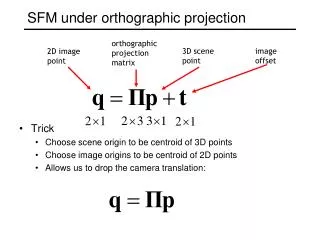
SFM under orthographic projection. Trick Choose scene origin to be centroid of 3D points Choose image origins to be centroid of 2D points Allows us to drop the camera translation:. orthographic projection matrix. 3D scene point. image offset. 2D image point.

E N D
SFM under orthographic projection • Trick • Choose scene origin to be centroid of 3D points • Choose image origins to be centroid of 2D points • Allows us to drop the camera translation: orthographic projection matrix 3D scene point image offset 2D image point
projection of n features in m images W measurement M motion S shape Key Observation: rank(W) <= 3 factorization (Tomasi & Kanade) projection of n features in one image:
solve for known • Factorization Technique • W is at most rank 3 (assuming no noise) • We can use singular value decomposition to factor W: • S’ differs from S by a linear transformation A: • Solve for A by enforcing metric constraints on M Factorization
Trick (not in original Tomasi/Kanade paper, but in followup work) • Constraints are linear in AAT : • Solve for G first by writing equations for every Pi in M • Then G = AAT by SVD Metric constraints • Orthographic Camera • Rows of P are orthonormal: • Enforcing “Metric” Constraints • Compute A such that rows of M have these properties
Extensions to factorization methods • Paraperspective [Poelman & Kanade, PAMI 97] • Sequential Factorization [Morita & Kanade, PAMI 97] • Factorization under perspective [Christy & Horaud, PAMI 96] [Sturm & Triggs, ECCV 96] • Factorization with Uncertainty [Anandan & Irani, IJCV 2002]
Structure from motion • How many points do we need to match? • 2 frames: (R,t): 5 dof + 3n point locations 4n point measurements n 5 • k frames: 6(k–1)-1 + 3n 2kn • always want to use many more CSE 576 (Spring 2005): Computer Vision
Bundle Adjustment • What makes this non-linear minimization hard? • many more parameters: potentially slow • poorer conditioning (high correlation) • potentially lots of outliers CSE 576 (Spring 2005): Computer Vision
Lots of parameters: sparsity • Only a few entries in Jacobian are non-zero CSE 576 (Spring 2005): Computer Vision
Robust error models • Outlier rejection • use robust penalty appliedto each set of jointmeasurements • for extremely bad data, use random sampling [RANSAC, Fischler & Bolles, CACM’81] CSE 576 (Spring 2005): Computer Vision
Structure from motion: limitations • Very difficult to reliably estimate metricstructure and motion unless: • large (x or y) rotation or • large field of view and depth variation • Camera calibration important for Euclidean reconstructions • Need good feature tracker • Lens distortion CSE 576 (Spring 2005): Computer Vision
Issues in SFM • Track lifetime • Nonlinear lens distortion • Prior knowledge and scene constraints • Multiple motions
Track lifetime every 50th frame of a 800-frame sequence
Track lifetime lifetime of 3192 tracks from the previous sequence
Track lifetime track length histogram
Nonlinear lens distortion effect of lens distortion
Prior knowledge and scene constraints add a constraint that several lines are parallel
Prior knowledge and scene constraints add a constraint that it is a turntable sequence
PhotoSynth http://labs.live.com/photosynth/
So far focused on 3D modeling • Multi-Frame Structure from Motion: • Multi-View Stereo Unknown camera viewpoints
Next • Recognition
Today • Recognition
Recognition problems • What is it? • Object detection • Who is it? • Recognizing identity • What are they doing? • Activities • All of these are classification problems • Choose one class from a list of possible candidates
How do human do recognition? • We don’t completely know yet • But we have some experimental observations.
Observation 1: The “Margaret Thatcher Illusion”, by Peter Thompson
Observation 1: • http://www.wjh.harvard.edu/~lombrozo/home/illusions/thatcher.html#bottom • Human process up-side-down images separately The “Margaret Thatcher Illusion”, by Peter Thompson
Observation 2: Kevin Costner Jim Carrey • High frequency information is not enough
Observation 3: • Negative contrast is difficult
Observation 4: • Image Warping is OK
The list goes on • Face Recognition by Humans: Nineteen Results All Computer Vision Researchers Should Know About http://web.mit.edu/bcs/sinha/papers/19results_sinha_etal.pdf
Face detection • How to tell if a face is present?
One simple method: skin detection • Skin pixels have a distinctive range of colors • Corresponds to region(s) in RGB color space • for visualization, only R and G components are shown above skin • Skin classifier • A pixel X = (R,G,B) is skin if it is in the skin region • But how to find this region?
Skin classifier • Given X = (R,G,B): how to determine if it is skin or not? Skin detection • Learn the skin region from examples • Manually label pixels in one or more “training images” as skin or not skin • Plot the training data in RGB space • skin pixels shown in orange, non-skin pixels shown in blue • some skin pixels may be outside the region, non-skin pixels inside. Why?
Skin classification techniques • Skin classifier • Given X = (R,G,B): how to determine if it is skin or not? • Nearest neighbor • find labeled pixel closest to X • choose the label for that pixel • Data modeling • fit a model (curve, surface, or volume) to each class • Probabilistic data modeling • fit a probability model to each class
Probability • Basic probability • X is a random variable • P(X) is the probability that X achieves a certain value • or • Conditional probability: P(X | Y) • probability of X given that we already know Y • called a PDF • probability distribution/density function • a 2D PDF is a surface, 3D PDF is a volume continuous X discrete X
Choose interpretation of highest probability • set X to be a skin pixel if and only if Where do we get and ? Probabilistic skin classification • Now we can model uncertainty • Each pixel has a probability of being skin or not skin • Skin classifier • Given X = (R,G,B): how to determine if it is skin or not?
Approach: fit parametric PDF functions • common choice is rotated Gaussian • center • covariance • orientation, size defined by eigenvecs, eigenvals Learning conditional PDF’s • We can calculate P(R | skin) from a set of training images • It is simply a histogram over the pixels in the training images • each bin Ri contains the proportion of skin pixels with color Ri This doesn’t work as well in higher-dimensional spaces. Why not?
Learning conditional PDF’s • We can calculate P(R | skin) from a set of training images • It is simply a histogram over the pixels in the training images • each bin Ri contains the proportion of skin pixels with color Ri • But this isn’t quite what we want • Why not? How to determine if a pixel is skin? • We want P(skin | R) not P(R | skin) • How can we get it?
what we measure (likelihood) domain knowledge (prior) what we want (posterior) normalization term Bayes rule • In terms of our problem: • The prior: P(skin) • Could use domain knowledge • P(skin) may be larger if we know the image contains a person • for a portrait, P(skin) may be higher for pixels in the center • Could learn the prior from the training set. How? • P(skin) may be proportion of skin pixels in training set
in this case , • maximizing the posterior is equivalent to maximizing the likelihood • if and only if • this is called Maximum Likelihood (ML) estimation Bayesian estimation • Bayesian estimation • Goal is to choose the label (skin or ~skin) that maximizes the posterior • this is called Maximum A Posteriori (MAP) estimation likelihood posterior (unnormalized) = minimize probability of misclassification • Suppose the prior is uniform: P(skin) = P(~skin) = 0.5
H. Schneiderman and T.Kanade General classification • This same procedure applies in more general circumstances • More than two classes • More than one dimension • Example: face detection • Here, X is an image region • dimension = # pixels • each face can be thoughtof as a point in a highdimensional space H. Schneiderman, T. Kanade. "A Statistical Method for 3D Object Detection Applied to Faces and Cars". IEEE Conference on Computer Vision and Pattern Recognition (CVPR 2000) http://www-2.cs.cmu.edu/afs/cs.cmu.edu/user/hws/www/CVPR00.pdf