Download
1 / 31
310 likes | 511 Views
One-digit industry wage structure in British Household Panel Survey data (Waves One to Eleven; N = 63 000). Average sample wage = £1163 per month (in real 1996 Pounds). Standard Industrial Classification Divisions: 0 Agriculture, forestry & fishing (£902) Energy & water supplies (£1758)

E N D
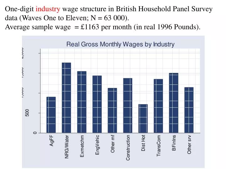
One-digit industry wage structure in British Household Panel Survey data (Waves One to Eleven; N = 63 000). Average sample wage = £1163 per month (in real 1996 Pounds).
Standard Industrial Classification Divisions: • 0 Agriculture, forestry & fishing (£902) • Energy & water supplies (£1758) • Extraction of minerals & ores other than fuels; manufacture of metals, mineral products & chemicals (£1544) • Metal goods, engineering & vehicles industries (£1435) • Other manufacturing industries (£1124) • Construction (£1371) • Distribution, hotels & catering (repairs) (£717) • Transport & communication (£1347) • Banking, finance, insurance, business services & leasing (£1499) • Other services (£1144)
One-digit occupational wage structure in British Household Panel Survey data (Waves One to Eleven; N = 63 000). Average sample wage = £1163 per month (in real 1996 Pounds).
Standard Occupational Classification Major Groups: 1 Managers & administrators (£1947) 2 Professional occupations (£1793) 3 Associate professional & technical occupations (£1457) 4 Clerical & secretarial occupations (£878) 5 Craft & related occupations (£1206) 6 Personal & protective service occupations (£728) 7 Sales occupations (£633) 8 Plant & machine operatives (£1131) 9 Other occupations (£647) For comparison: Non-union (£1093) Union (£1377) Female (£862) Male (£1491)
Observation: There are industry and occupational wage differentials. Question: Are these rents or compensating differentials?or: Are high-wage jobs “better” than low-wage jobs? Data: Eleven waves of the British Household Panel Survey (BHPS). Method: Two stages. Correlate the estimated occupational coefficients from a wage equation with those from a utility (job satisfaction) equation. A positive correlation implies that (inexplicably) high-wage occupations are also (inexplicably) high satisfaction occupations, which sounds like rents. The same approach for the industry coefficients. LOOKING FOR LABOUR MARKET RENTS WITH SUBJECTIVE DATAAndrew E. Clark (PSEand IZA)
Results: OCCUPATION coefficients are POSITIVELY AND SIGNIFICANTLY correlated: especially for younger workers and for men. However, there are NO SIGNIFICANT CORRELATIONS at the INDUSTRY level.This result holds for both level and panel first-stage regressions.Interpretation: Occupational wage differences are partly rents; industry wage differences are not.
Supporting evidence: Use spell data. How do individuals get to the high-rent occupations?* From EMPLOYMENT (no surprise).* Via PROMOTION, rather than via voluntary mobility.* There is evidence of JOB-QUALITY LADDERS at the firm level.
Conclusion: • There are occupational rents. They aren’t competed away because firms control access to them, rather than workers. • Why do firms allow rents to exist? Perhaps to incite effort, as in tournament theory (evidence of job ladders) • Firms can only supply tournaments across occupations, not across industries. The industry wage structure then likely reflects other phenomena.
Wage and job satisfaction regressions.The utility function of worker i in occupation o, Uio, is assumed to be linear in wages, job disamenities, Do, and a raft of other individual and job characteristics, Xi: Uio = ’Xi + wio - Dio (1)The compensating differential offered by firms for Do will be just enough to keep the worker on the same indifference curve: a unit of D is compensated by extra income of / .
The wage of worker i in occupation o is argued, for simplicity, to depend on the same X’s as does utility in (1), compensation for the disamenities in that occupation, Do, and an occupation specific rent, o: • wio = ’Xi + o + βDo (2) • Note that worker homogeneity is assumed. From the utility function, the compensating differential for D is β=/. • Substituting for wio and β in (1) yields • Uio = ’Xi + o (3)
I estimate equations (2) and (3). I have no information on o or Do: these are picked up by two-digit occupational and industry dummies. In the wage equation, the estimated coefficients on these dummies will pick up both rents and disamenities (o + βDo); in the utility (job satisfaction) equation, the estimated coefficients will only reflect rents (o). The empirical strategy is therefore to see if the systematic differences in utility/job satisfaction across occupations are correlated with their counterparts in a standard wage equation. Correlate: the estimate of o + βDo with that of o. Strong correlation => the rent component of wage differentials is substantial. Weak correlation => the rent element, o, is small.
Data BHPS Waves 1 to 11. Employees 16 to 65 only: 27 000 observations; 7000 different individuals. [http://www.iser.essex.ac.uk/bhps] The proxy utility measure is overall job satisfaction (which predicts quits, absenteeism, and productivity). Measured on a one to seven scale:
BHPS: Overall Job Satisfaction Value Frequency Percentage Not Satisfied at All 1 521 1.9% 2 772 2.9% 3 1966 7.3% 4 2177 8.1% 5 5718 21.3% 6 11595 43.2% Completely Satisfied 7 4088 15.2% ‑‑‑‑‑- ‑‑‑‑‑‑-- Total 26837 100.0%
Figure 1. The Relation between Estimated Coefficients in Wage and Job Satisfaction Regressions (Results for Men)
Figure 1. The Relation between Estimated Coefficients in Wage and Job Satisfaction Regressions (Results for Men)
Figure 1. The Relation between Estimated Coefficients in Wage and Job Satisfaction Regressions (Results for Men)
Figure 1. The Relation between Estimated Coefficients in Wage and Job Satisfaction Regressions (Results for Men)
Note: Bold = significant at the five per cent level; Italic = significant at the ten per cent level.
INTERPRETATIONS Omitted variables (ability, unemployment rate etc) • The same results are found in both panel and level regressions • Controlling for the local unemployment rate doesn’t change anything. • Controlling for thirteen-level education doesn’t either.
INTERPRETATIONS Endogenous choice of occupation/heterogeneity • Panel results are the same as level results. • If there is sorting, we’d expect higher correlations for older workers (who have already sorted): we find the opposite. • Try and control for tastes for income and hard work: • marital status, number and ages of children, spouse’s labour force status, spouse’s income. • Parents’ labour force status, parents’ occupation. • A number of these attract significant estimates, but the correlation between the occupation coefficients in wage and job satisfaction regressions stays the same, as does that for industry coefficients.
I think that the occupational differences reflect rents..... Here’s why: Table 3. Getting to the Good Jobs: Occupations Use BHPS Spell data to see how individuals get to not high and high-quality jobs (as defined by negative or insignificant, and positive significant occupation dummy estimates in Table 1's job satisfaction regressions respectively).