Download
1 / 64
680 likes | 1.05k Views
Parametrization of the planetary boundary layer (PBL) Peter Baas Many thanks to Anton Beljaars & Martin Köhler. Introduction. Outer layer. Surface layer and surface fluxes. KNMI ECMWF course – 16 june 2010. Los Angeles PBL. July 2001. Downtown LA. PBL top. 10km. Griffith Observatory.

E N D
Parametrization of the planetary boundary layer (PBL)Peter BaasMany thanks to Anton Beljaars & Martin Köhler • Introduction. • Outer layer. • Surface layer and surface fluxes. KNMI ECMWF course – 16 june 2010
Los Angeles PBL July 2001 Downtown LA PBL top 10km Griffith Observatory 1000 to 10000 die annually in LA from heart disease resulting from SMOG.
Boundary layer: definition The PBL is the layer close to the surface within which vertical transports by turbulence play dominant roles in the momentum, heat and moisture budgets. Turbulent flows are characterized by fluctuating dynamical quantities in space and time in a “disordered” manner (Monin and Yaglon, 1973). Turbulent motion is small-scale and totally sub-grid and therefore needs to be parameterized.
Space and time scales • Diffusive transport in the atmosphere is dominated by turbulence. • Time scale of turbulence varies from seconds to half hour. • Length scale varies from mm for dissipative eddies to 100 m for transporting eddies. • The largest eddies are the most efficient ones for transport. cyclones microscale turbulence diurnal cycle spectral gap 100 hours 1 hour 0.01 hour data: 1957
T-tendencies due to turbulencescheme [K/day] Jan. 1999
U-Profile … Effects of Terrain z0~1-10cm z0~50cm z0~1m Ocean: z0~0.1-1mm Neutral: Oke 1978
U-Profile … Effects of Stability Neutral Stable Height ln (Height) surface layer Unstable Neutral: Oke 1978
Diurnal cycle of boundary layer Free Atmosphere Residual Layer Convective Mixed Layer Stable (nocturnal) Boundary Layer Noon Sunset Midnight Sunrise Noon convective BL convective BL stable BL Surface Layer
Diurnal cycle of profiles convective BL stable BL Oke 1978
Conserved variables For turbulent transport in the vertical, quantities are needed that are conserved for adiabatic ascent/descent. For dry processes: pot. temperature dry static energy For moist processes: liq. wat. pot. temperature liq. water static energy total water
Buoyancy parameter unstable stable To determine static stability, move a fluid parcel adiabatically in the vertical and compare the density of the parcel with the density of the surrounding fluid. Virtual potential temperature and virtual dry static energy are suitable parameters to describe stability: Virtual temperature: temperature dry air would have if pressure and density were equal to given sample of moist air.
Part 2: The Outer Layer • Basic equations and the closure problem • Overview of models • Local K closure • K-Profile closure • EDMF • TKE closure “Everything above the lowest model level”
TENDENCY ADVECTION ROTATION PRESSURE GRADIENT VISCOUS STRESS GRAVITY Basic equations mom. equ.’s continuity How to incorporate sub-grid scale motions?
Reynolds decomposition Substitute, apply averaging operator. Averaging (overbar) is over grid box, i.e. sub-grid turbulent motion is averaged out. Property of averaging operator: E.g.
Assumptions… Reynold’s decomposition Boussinesq approximation (density in buoyancy terms only) and Hydrostatic approximation (vertical acceleration << buoyancy). Boundary layer approximation (horizontal scales >> vertical scales), e.g. : High Reynolds number approximation (molecular diffusion << turbulent transports), e.g.:
Reynolds equations The 2nd order correlations are unknown (closure problem) and need to be parametrized (i.e. expressed in terms of large scale variables). Reynolds Terms
Solving the closure problem… K-diffusion method: analogous to molecular diffusion Next question: how to parametrize K? Stull (1988): “There has been no lack of creativity by investigators in designing parameterizations for K”
ECMWF PBL regimes K profile EDMF Local K TKE
Parametrization of PBL outer layer • local K closure • K-profile closure • EDMF • TKE closure
local K closure model: Grid point models Levels in ECMWF model K-diffusion in analogy with molecular diffusion, but 91-level model 31-level model Diffusion coefficients need to be specified as a function of flow characteristics (e.g. shear, stability, length scales).
Flux-gradient relations (stability functions) fm fh m h Bus-Dyer z/L – dimensionless shear – dimensionless lapse rate z/Λ • Follow from Monin-Obukhov Similarity Theory • Relate profiles of mean quantities to turbulent fluxes • All dimensionless parameters unique function of stability parameter z/L, where L is the Obukhov length. • Semi-empirical, because based on dimensional analysis and observations • Corrects neutral K for stability Application :
Diffusion coefficients according to MO-similarity Problem: closure is implicit Use relation between and to solve for . IFS generates look-up table with z/L = f (Ri )
K-closure with local stability dependence (summary) Alternatively, use instead of • Scheme is simple and easy to implement. • Fully consistent with local scaling for stable boundary layer. • A sufficient number of levels is needed to resolve the BL i.e. to locate inversion.
Model sensitivity to stability functions z/L More mixing! Unfortunately, realistic stability functions have detrimental effect on 500hPa scores.
Parametrization of PBL outer layer • local K-closure • K-profile closure • EDMF • TKE closure
K-profile closure Troen and Mahrt (1986) h Heat flux Profile of diffusion coefficients: Find inversion by parcel lifting with T-excess: such that:
K-profile closure (ECMWF up to 2005) • Inversion interaction was too aggressive in original scheme and too much dependent on vertical resolution. • Features of ECMWF implementation: • No counter gradient terms. • Not used for stable boundary layer. • Lifting from minimum virtual T. • Different constants. • Implicit entrainment formulation. Entrainment fluxes h Moisture flux Heat flux ECMWF entrainment formulation: ECMWF Troen/Mahrt C1 0.6 0.6 D 2.0 6.5 CE 0.2 - or
K-profile closure (summary) • Scheme is simple and easy to implement. • Numerically robust. • Scheme simulates realistic mixed layers. • Counter-gradient effects can be included (might create numerical problems). • Entrainment can be controlled rather easily. • A sufficient number of levels is needed to resolve BL e.g. to locate inversion.
Parametrization of PBL outer layer • Overview of models • local K-closure • K-profile closure • EDMF • TKE closure
Eddy-Diffusivity – Mass Flux (EDMF) ECMWF since 2005 • Decomposes turbulent flux into a part that includes strong organized updraughts and a remaining turbulence field. • Combines diffusion and mass-flux: local non-local transport K-profile Siebesma et al. (2007)
Parametrization of PBL outer layer • Overview of models • local K closure • K-profile closure • TKE closure
TKE closure (1.5 order) Eddy diffusivity approach: With diffusion coefficients related to kinetic energy:
Closure of TKE equation Pressure correlation TKE from prognostic equation: Storage Shear production Buoyancy Turbulent transport Dissipation with closure: Main problem is specification of length scales, which are usually a blend of , an asymptotic length scale and a stability related length scale in stable situations.
TKE (summary) Best to implement TKE on half levels. • TKE has natural way of representing entrainment. • One scheme for all regimes. • TKE needs more resolution than first order schemes. • TKE does not necessarily reproduce MO-similarity.
TKE closure vs 1st order closure for stable conditions TKE closure vs 1st order closure for stable conditions z/L A More mixing! B C C B A Contours: Length scale for stable: B C A
Parameterization PBL, the calltree General master1c … suphec1c(setup routine for constants in modules) callpar (controls computation of physical tendencies) | vdfouter(calls vdfmain 2 times with ½ of the normal time step) | vdfmain(physical tendencies by vertical diffusion) suphec1c | susurf … susveg (sets vegetation parameters for tiles, eg roughness length tables) | suvdfs (setup routine for constants and tables related to stability functions, eg Ri vs z/L table) | fcvds (define stability functions) vdfmain Surface | surfexcdriver (controls routines that deal with surface exchange coefficients and associated quantities) | vupdz0 (computes roughness length over ocean and sets over land) | vexcs (determines transfer coefficients, solves for L by iteration) | vsflx (computes surface fluxes) Outer layer | vdfhghtn (determines updraught properties and inversion height) | vdfexcu (determines turbulent diffusion coefficients between model levels above surface layer)
Part 3: The Surface Layer and Surface Fluxes • Surface layer (Monin Obukhov) similarity • Surface flux formulation • Roughness length over land • Ocean surface fluxes “Between the lowest model level and the surface”
Surface layer • Also called ‘constant-flux layer’ • In practice between lowest model level and surface • Mixing across steep gradients Stable BL Dry mixed layer Cloudy BL Surface flux parametrization is sensitive because of large gradients near the surface.
Boundary conditions for T and q have different character over land and ocean Surface fluxes of heat and moisture are proportional to temperature and moisture differences: Lowest model level T1,q1 z1 Ts, qs Surface Ocean boundary condition Land boundary condition
Parametrization of surface fluxes: Outline • Surface layer (Monin Obukhov) similarity • Surface flux formulation • Roughness length over land • Ocean surface fluxes
Surface layer similarity (Monin Obukhov similarity) For z/h << 1 flux is approximately equal to surface flux. Flux profile • Considerations about the nature of the process: • z/zo >> 1 • distance to surface determines turbulence length scale • shear scales with surface friction rather than with zo Scaling parameters:
MO similarity for gradients is a universal function of dimensionless shear Stability parameter is a universal function of dimensionless potential temperature gradient Stability parameter Note that with we obtain:
MO gradient functions Observations of as a function of z/L, with Empirical gradient functions to describe these observations: unstable stable
Parametrization of surface fluxes: Outline • Surface layer (Monin Obukhov) similarity • Surface flux formulation • Roughness length over land • Ocean surface fluxes
Integral profile functions for momentum Dimensionless wind gradient (shear) or temperature gradient functions can be integrated to profile functions: with: integration constant (roughness length for momentum) wind profile function, related to gradient function: Profile functions for temperature and moisture can be obtained in similar way.
Integral profile functions: Momentum, heat and moisture Profile functions for surface layer applied between surface and lowest model level provide link between fluxes and differences of wind, temperature and moisture.
MO wind profile functions applied to observations Unstable Stable Holtslag, 1984
Transfer coefficients Surface fluxes can be written explicitly as: Lowest model level U1,V1,T1,q1 z1 0, 0, Ts, qs Surface