Download
1 / 42
420 likes | 512 Views
Cooperative Control and Mobile Sensor Networks Cooperative Control, Part I, D-F. Naomi Ehrich Leonard Mechanical and Aerospace Engineering Princeton University and Electrical Systems and Automation University of Pisa

E N D
Cooperative Control and Mobile Sensor Networks Cooperative Control, Part I, D-F Naomi Ehrich Leonard Mechanical and Aerospace Engineering Princeton University and Electrical Systems and Automation University of Pisa naomi@princeton.edu, www.princeton.edu/~naomi
Outline and Key References Artificial Potentials and Projected Gradients: R. Bachmayer and N.E. Leonard. Vehicle networks for gradient descent in a sampled environment. In Proc. 41st IEEE CDC, 2002. Artificial Potentials and Virtual Beacons: N.E. Leonard and E. Fiorelli. Virtual leaders, artificial potentials and coordinated control of groups. In Proc. 40th IEEE CDC, pages 2968-2973, 2001. Artificial Potentials and Virtual Bodies with Feedback Dynamics: P. Ogren, E. Fiorelli and N.E. Leonard. Cooperative control of mobile sensor networks: Adaptive gradient climbing in a distributed environment. IEEE Transactions on Automatic Control, 49:8, 2004.
Outline and Key References D. Virtual Tensegrity Structures: B. Nabet and N.E. Leonard. Shape control of a multi-agent system using tensegrity structures. In Proc. 3rd IFAC Wkshp on Lagrangian and Hamiltonian Methods for Nonlinear Control, 2006. E. Networks of Mechanical Systems and Rigid Bodies: S. Nair, N.E. Leonard and L. Moreau. Coordinated control of networked mechanical systems with unstable dynamics. In Proc. 42nd IEEE CDC, 2003. T.R. Smith, H. Hanssmann and N.E. Leonard. Orientation control of multiple underwater vehicles. In Proc. 40th IEEE CDC, pages 4598-4603, 2001. S. Nair and N.E. Leonard. Stabilization of a coordinated network of rotating rigid bodies. In Proc. 43rd IEEE CDC, pages 4690-4695, 2004. F. Curvature Control and Level Set Tracking: F. Zhang and N.E. Leonard. Generating contour plots using multiple sensor platforms. In Proc. IEEE Swarm Intelligence Symposium, 2005.
D. Virtual Tensegrity Structures with Ben Nabet
Linear Model (see papers by R. Connelly) Real cables do not increase in length and real struts do not decrease in length.
Equilibria This fixes the shape of the equilibria but not the size.
Shape Change Choose a path from initial to final configuration that consists of a path of stable tensegrity structures. Can then prove boundedness of transient and convergence to final structure.
Cable Strut Initial shape Final shape
Geometric framework: Method of Controlled Lagrangians • with A.M. Bloch and J.E. Marsden • - Energy shaping for stabilization of (otherwise unstable) • underactuated mechanical systems. • - Restrict to control dynamics that derive from a Lagrangian. • - Theory is constructive for certain classes: Synthesis! • also D.E. Chang and C.A. Woolsey, • P.S. Krishnaprasad, G. Sanchez de Alvarez, • see also IDA-PBC method – Blankenstein, Ortega, Spong, van der Schaft et al E. Networks of Mechanical Systems/Rigid Bodies
Method of Controlled Lagrangians • Given a mechanical system, possibly underactuated and possibly with unstable dynamics. • Design Lcso corresponding Euler-Lagrange equations match original equations with control law. • Matching conditions are PDE’s. • For certain classes of systems, use structured modification Lc of L • - Q=S x G. L invariant to G. Shape kinetic energy metric. • - Modify potential energy to break symmetry (if desired). • Yields parametrized family of Lc that satisfy matching conditions. • Theory provides conditions on (control) parameters for stability: m f g l - Construct energy function. - Consider dissipation and asymptotic stability u M s Bloch, Leonard, Marsden, IEEE TAC, 2000, 2001
Coordination • Design artificial potentials to couple N individual systems. • - Relative position/orientation of vehicle pairs. • - Potential well = desired group configuration. • Treat coupled multi-body system with same approach as for individual. • - Symmetry group G for Hamiltonian + potentials. • - Reduce action of G on phase space. • - Construct energy function to prove: • Individual dynamics are stabilized and group is stably coordinated. Nair and Leonard; Smith, Hanssmann and Leonard
N times Role of Symmetry • Potentials will break symmetry: • E.g., consider N vehicles and Q = SE(3) x . . . x SE(3) • Suppose Q is original symmetry group. • - Break N-1 copies of SO(3) to align orientations. • - Break N-1 copies of SE(3) to align and distribute. • - Break N copies of SO(3) to align and to orient whole group, etc. • Break symmetry for coordination and group cohesion. • Preserve symmetries when control authority is limited. • Discrete symmetries in homogeneous group with no ordering.
Same Features as in Particle Systems • Distributed control. • Neighborhood of each vehicle can be prescribed. • (Global info not required) • No ordering of vehicles is necessary. Provides robustness to failure. • Vehicles are interchangeable. Illustrations: A. Two (underwater) vehicles in SE(3) B. N inverted-pendulum-on-cart systems.
B A A B A: Coordinated Orientation of 2 Vehicles in SE(3) with Troy Smith and Heinz Hanssmann
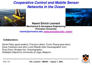
B: Coordination of Mechanical Systems with Unstable Dynamics with Sujit Nair • Extend controlled Lagrangians to collection of unstable • mechanical systems with controlled coupling. • Class of systems includes inverted pendulum on a cart. • Goal: Stabilize each pendulum in the upright position while • synchronizing the motion of the carts.
m f g l M u s c sin f y Extension to Network of Systems
Exploring Scalar Fields Curvature Control and Level Set Tracking Generating a contour plot with three clusters: Fumin Zhang and N.E. Leonard, Proc. IEEE Swarm Symposium, 2005
Filter Design Four moving sensor platforms, each takes one measurement a time: Taylor Series:
Filter Design Filtering problem: From a series of measurements find and at the center. Step k-1: Step k:
Filter Design Prediction: Step k-1: Step k:
Filter Design Update: Find that minimizes error covariance of prediction error covariance of measurements We get:
Filter Design Estimate: A special arrangement to simplify the estimators
Filter Design Estimate: How to estimate the Hessian We have a prediction
Filter Design Estimate: Assuming formation is small enough
Filter Design We now know the Hessian:
Formation Design Estimation Error: Error in estimate of field value at center. Error in estimate of gradient at center. Optimization: Find and that minimize the mean square error L.
Formation Design Optimization: Covariance matrix of updated measurements Error in estimate of first diag. el. of Hessian General solutions are numerical. We found analytical solutions when Bis diagonal. [Ögren, Fiorelli and Leonard 04],[FZ, Leonard SIS05][FZ, Leonard CDC06].
Cooperative Control Goals for cooperative controllers: • Achieve the cross formation with optimal shape and . • Align the horizontal axis of the formation with the tangent vector to the level curve at the center. • Control the motion of the center to go along the desired level curve. We get a contour plot with gradient estimates along the level curve.
Cooperative Control Jacobi Vectors:
Cooperative Control Decoupled Dynamics: Formation Center where and
Cooperative Control Formation Control:
Tracking Level Curves Reduced center dynamics: Boundary tracking is a special case.
Tracking Level Curves Control Lyapunov Function: Steering Control: which achieves Convergence proved using LaSalle’s Invariance Principle. [FZ, Leonard CDC06, SIS05]