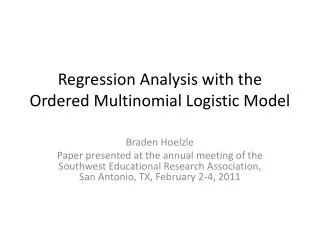
Regression Analysis with the Ordered Multinomial Logistic Model
Regression Analysis with the Ordered Multinomial Logistic Model. Braden Hoelzle Southern Methodist University December 2009. Situating the Model. Review: Logistic Regression. Dichotomous Dependent Variable Independent Variables can be dichotomous, integral, categorical…etc.

Regression Analysis with the Ordered Multinomial Logistic Model
E N D
Presentation Transcript
Regression Analysis with the Ordered Multinomial Logistic Model Braden Hoelzle Southern Methodist University December 2009
Review: Logistic Regression • Dichotomous Dependent Variable • Independent Variables can be dichotomous, integral, categorical…etc. • We are trying to predict the probability that a person does or doesn’t have a trait • Example: At risk of dropping out or Not at risk • Others??
Transform to Probability • Probability range = (0 ≤ p ≥ 1) • Therefore we must transform continuous values to the range 0-1 by using the formula: Or expanded to:
A Quick Example > m1 <- glm(comply ~ physrec, family = binomial(link = "logit")) > summary(m1) Call: glm(formula = comply ~ physrec, family = binomial(link = "logit")) Coefficients: Estimate Std. Error z value Pr(>|z|) (Intercept) -1.8383 0.4069 -4.518 6.26e-06 physrec 2.2882 0.4503 5.081 3.75e-07 The probability of complying if NOT recommended by physician: • exp(-1.8383)/(1 + exp(-1.8383)) 0.1372525 The probability of complying if recommended by physician: • exp(-1.8383 + 2.2882)/(1 + exp(-1.8383 + 2.2882)) 0.6106392
OrderedMultinomial Logistic Model Four Types of Scales 1. _________ - mutually exclusive categories w/ no logical order. 2. _________ - mutually exclusive categories w/ logical rank order. 3. _________ - ordered data w/ equal distance between each point (no absolute zero). 4. _________ - ordered data w/ equal distance between each point (w/ a “true” zero). What type of data would you expect our ordered multinomial regression to model?
Definition • The ordered multinomial logistic model enables us to model ordinally scaled dependent variables with one or more independent variables. • These IV(s) can take many different forms (ie. real numbers values, integers, categorical, binomial, etc.).
Does this Occur Much? “Ordinal data are the most frequently encountered type of data in the social sciences” (Johnson & Albert, 1999, p. 126). • Examples • Yes, maybe, no • Likert scale (Strongly Agree – Strongly Disagree) • Always, frequently, sometimes, rarely, never • No hs diploma, hs diploma, some college, bachelor’s degree, master’s degree, doctoral degree • Free school lunch, reduced school lunch, full price lunch • 0-10k per year, 10-20K per year, 20-30K per year, 30 – 60K per year, > 60K per year • Low, medium, high • Basic math, regular math, pre-AP math, AP math • Nele’s dancing ability, Meg’s dancing ability, Saralyn’sdancing ability, Jose’s dancing ability, Kyle’s dancing ability, Braden’s dancing ability, a rock
Running Regression using the Ordered Multinomial Logistic Model in R Load/Install Libraries: library(arm) library (psych) Load data (UCLA – Academic Technology Services, n.d.) mydata <- read.csv(url("http://www.ats.ucla.edu/st at/r/dae/ologit.csv")) attach(mydata)
Definitions Variables: apply- college juniors reported likelihood of applying to grad school (0 = unlikely, 1 = somewhat likely, 2 = very likely) pared – indicating whether at least one parent has a graduate degree (0 = no, 1 = yes) public – indicating whether the undergraduate institution is a pubic or private (0 = private, 1 = public) gpa – college gpa Which variable will likely be our dependent variable?
Description of Data > str(mydata) 'data.frame': 400 obs. of 4 variables: $ apply : int 2 1 0 1 1 0 1 1 0 1 ... $ pared : int 0 1 1 0 0 0 0 0 0 1 ... $ public: int 0 0 1 0 0 1 0 0 0 0 ... $ gpa : num 3.26 3.21 3.94 2.81 2.53 ... > summary(mydata$gpa) Min. 1st Qu. Median Mean 3rd Qu. Max. 1.900 2.720 2.990 2.999 3.270 4.000 > table(apply) apply 0 1 2 220 140 40 > table(pared) pared 0 1 337 63 > table(public) public 0 1 343 57
Crosstabs > xtabs(~ pared + apply) apply pared 0 1 2 0 200 110 27 1 20 30 13 > xtabs(~ public + apply) apply public 0 1 2 0 189 124 30 1 31 16 10 Why would this information be important for running our ordered multinomial logistic model?
Assumptions No perfect predictions – one predictor variable value cannot solely correspond to one dependent variable value. (ex. – Every student w/ parents who went to graduate school cannot indicate that they are very likely to attend graduate school) – check using crosstabs ( see slide 12). No empty or very small cells – see crosstabs. Sample Size – always requires more cases than OLS regression.
Running a Single Predictor Model > summary(m1 <- bayespolr(as.ordered(apply)~gpa,data=mydata)) Call: bayespolr(formula = as.ordered(apply) ~ gpa, data = mydata) Coefficients: Value Std. Error t value gpa 0.7109826 0.247078 2.877563 Intercepts: Value Std. Error t value 0|1 2.3308 0.7502 3.1068 1|2 4.3508 0.7744 5.6183 Residual Deviance: 737.6921 AIC: 743.6921
Transforming Outcomes to Probabilities • (beta <- coef(m1)) gpa 0.7109826 • (tau <- m1$zeta) 0|1 1|2 2.330831 4.350816 • x<- 3 ##### Note: mean = 2.999 • logit.prob <- function(eta){exp(eta)/(1+exp(eta))} • (p1 <- logit.prob(tau[1] - x * beta)) 0.54931 • (p2<- logit.prob(tau[2] - x * beta) - logit.prob(tau[1] - x * beta)) 0.3525327 • (p3<- 1 - logit.prob(tau[2] - x * beta)) 0.09815732 • p1+p2+p3 1
Adding Multiple Predictors > summary(m2 <- bayespolr(as.ordered(apply)~gpa + pared + public ,data=mydata)) Call: bayespolr(formula = as.ordered(apply) ~ gpa + pared + public, data = mydata) Coefficients: Value Std. Error t value gpa 0.6041463 0.2577039 2.3443424 pared 1.0274106 0.2636348 3.8970973 public -0.0528103 0.2931885 -0.1801240 Intercepts: Value Std. Error t value 0|1 2.1638 0.7710 2.8064 1|2 4.2518 0.7955 5.3449 Residual Deviance: 727.002 AIC: 737.002
Transforming Outcomes to Probabilities • (beta <- coef(m2)) gpa pared public 0.6041463 1.0274106 -0.0528103 • (tau <- m2$zeta) 0|1 1|2 2.163841 4.251774 • (x<- cbind(0:4, 0 , .15)) [,1] [,2] [,3] [1,] 0 0 0.15 [2,] 1 0 0.15 [3,] 2 0 0.15 [4,] 3 0 0.15 [5,] 4 0 0.15 • (x2<-cbind(0:4, 1 , .15)) [,1] [,2] [,3] [1,] 0 1 0.15 [2,] 1 1 0.15 [3,] 2 1 0.15 [4,] 3 1 0.15 [5,] 4 1 0.15
Transforming Outcomes to Probabilities (cont.) • logit.prob <- function(eta){exp(eta)/(1+exp(eta))} • (p1 <- logit.prob(tau[1] - x %*% beta)) [,1] [1,] 0.8976849 [2,] 0.8274435 [3,] 0.7238159 [4,] 0.5888766 [5,] 0.4390981 • (p2<- logit.prob(tau[2] - x %*% beta) - logit.prob(tau[1] - x %*% beta)) [,1] [1,] 0.08838526 [2,] 0.14736050 [3,] 0.23102713 [4,] 0.33148400 [5,] 0.42421801 • (p3<- 1 - logit.prob(tau[2] - x %*% beta)) [,1] [1,] 0.01392982 [2,] 0.02519605 [3,] 0.04515695 [4,] 0.07963941 [5,] 0.13668388
Transforming Outcomes to Probabilities (cont.) • (p4 <- logit.prob(tau[1] - x2 %*% beta)) [,1] [1,] 0.7584777 [2,] 0.6318601 [3,] 0.4840202 [4,] 0.3389252 [5,] 0.2188751 • (p5<- logit.prob(tau[2] - x2 %*% beta) - logit.prob(tau[1] - x2 %*% beta)) [,1] [1,] 0.2035536 [2,] 0.3007906 [3,] 0.3992730 [4,] 0.4663890 [5,] 0.4744476 • (p6<- 1 - logit.prob(tau[2] - x2 %*% beta)) [,1] [1,] 0.03796871 [2,] 0.06734929 [3,] 0.11670683 [4,] 0.19468576 [5,] 0.30667730
Why Not Use Linear Regression? > summary(m1.2<-lm(apply~gpa, data=mydata)) Call: lm(formula = apply ~ gpa, data = mydata) Residuals: Min 1Q Median 3Q Max -0.7917 -0.5554 -0.3962 0.4786 1.6012 Coefficients: Estimate Std. Error t value Pr(>|t|) (Intercept) -0.22016 0.25224 -0.873 0.38329 gpa 0.25681 0.08338 3.080 0.00221 ** --- Signif. codes: 0 ‘***’ 0.001 ‘**’ 0.01 ‘*’ 0.05 ‘.’ 0.1 ‘ ’ 1 Residual standard error: 0.6628 on 398 degrees of freedom Multiple R-squared: 0.02328, Adjusted R-squared: 0.02083 F-statistic: 9.486 on 1 and 398 DF, p-value: 0.002214
What Do Our Results Mean? Plug in a gpa of 3: > (y.hat<-(-.2201 + (.2568 * 3))) [1] 0.5503 This means that we expect someone w/ a 3.0 gpa to fall about half way between unlikely (0) and slightly likely (1) to apply to grad school. But what is half way between these two points (a little unlikely?, neither likely nor unlikely?, very slightly likely?) This is somewhat vague.
Our Graph using Linear Regression An OLS Line on Our Data A Normal OLS Line
However… The decision between linear regression and ordered multinomial regression is not always black and white. When you have a large number of categories that can be considered equally spaced simple linear regression is an optional alternative (Gelman & Hill, 2007). ** But check your assumptions!!
Practice Read in the following table (Quinn, n.d.): nes96 <- read.table("http://www.stat.washington.edu/quinn/classes/536/data/nes96r.dat", header=TRUE) Run a regression using the ordered multinomial logistic model to predict the variation in the dependent variable ClinLR using the dependent variables PID and educ. ClinLR = Ordinal variable from 1-7 indicating ones view of Bill Clinton’s political leanings, where 1 = extremely liberal, 2 = liberal, 3 = slightly liberal, 4 = moderate, 5= slightly conservative, 6 = conservative, 6 = extremely conservative. PID = Ordinal variable from 0-6 indicating ones own political identification, where 0 = Strong Democrat and 6 = Strong Republican educ= Ordinal variable from 1-7 indicating ones own level of education, where 1 = 8 grades or less and no diploma, 2 = 9-11 grades, no further schooling, 3 = High school diploma or equivalency test, 4 = More than 12 years of schooling, no higher degree, 5 = Junior or community college level degree (AA degrees), 6 = BA level degrees; 17+ years, no postgraduate degree, 7 = Advanced degree
References • Gelman, A. & Hill, J. (2007). Data analysis using regression and multilevel/hierarchical models. New York: Cambridge University Press. • Johnson, V. E. & Albert, J. H. (1999). Statistics for the social sciences and public policy: Ordinal data modeling. New York: Springer. • Quinn, K. (n.d.). Retrieved from http://www.stat.washington.edu/quinn/cl asses/536/data/nes96r.dat • UCLA: Academic Technology Services. (n.d.). Retrieved from http://www.ats.ucla.edu/st at/r/dae/ologit.csv