Statistics for Microarray Data Analysis with R

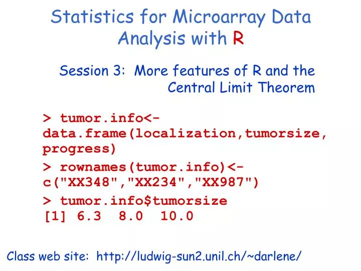
1. Statistics for Microarray Data Analysis with R Session 3: More features of R and the Central Limit Theorem > tumor.info<-data.frame(localization,tumorsize,progress) > rownames(tumor.info)<-c("XX348","XX234","XX987") > tumor.info$tumorsize • [1] 6.3 8.0 10.0 Class web site: http://ludwig-sun2.unil.ch/~darlene/

2. Today’s Outline • Further features of the R language • Preliminary data analysis exercise • Central Limit Theorem (CLT) • CLT exercise • some material included here was adapted from materials available at http://www.bioconductor.org/ and is used by permission

3. R: factors • Categorical variables in R should be specified as factors • Factors can take on a limited number of values, called levels • Levels of a factor may have a natural order • Functions in R for creating factors: factor(), ordered()

4. R:data frames (review) • data frame:the type of R object normally used to store a data set • A data frameis a rectangular table with rows and columns • data within each column has the same type (e.g. number, character, logical) • different columns may have different types • Example: > tumor.info localisation tumorsize progress XX348 proximal 6.3 FALSE XX234 distal 8.0 TRUE XX987 proximal 10.0 FALSE

5. R: making data frames • Data frames can be created in R by importing a data set • A data frame can also be created from pre-existing variables • Example: > localisation<-c("proximal","distal","proximal") > tumorsize<- c(6.3,8,10) > progress<-c(FALSE,TRUE,FALSE) > tumor.info<-data.frame(localization,tumorsize,progress) > rownames(tumor.info)<-c("XX348","XX234","XX987") > tumor.info$tumorsize [1] 6.3 8.0 10.0

6. R: more on subsetting > tumor.info[c(1,3),] localisation tumorsize progress XX348 proximal 6.3 FALSE XX987 proximal 10.0 FALSE > tumor.info[c(TRUE,FALSE,TRUE),] localisation tumorsize progress XX348 proximal 6.3 0 XX987 proximal 10.0 0 > tumor.info$localisation [1] "proximal" "distal" "proximal" > tumor.info$localisation=="proximal" [1] TRUE FALSE TRUE > tumor.info[ tumor.info$localisation=="proximal", ] localisation tumorsize progress XX348 proximal 6.3 0 XX987 proximal 10.0 0 subset rows by a vector of indices subset rows by a logical vector subset a column comparison resulting in logical vector subset the selected rows

7. R: loops • When the same or similar tasks need to be performed multiple times in an iterative fashion • A data frame can also be created from pre-existing variables • Examples: > for(i in 1:10) { > i = 1 print(i*i) while(i<=10) { } print(i*i) i=i+sqrt(i) } • Explicit loops such as these should be avoidedwhere possible

8. R:lapply, sapply • When the same or similar tasks need to be performed multiple times for all elements of a list or for all columns of an array • These implicit loops are generally faster than explicit ‘for’ loops • lapply(the.list,the.function) • the.function is applied to each element of the.list • result is a list whose elements are the individual results for the.function • sapply(the.list,the.function) • Like lapply, but tries to simplify the result, by converting it into a vector or array of appropriate size

9. R:apply • apply(array, margin,the.function) • applies the.function along the dimension of array specified by margin • result is a vector or matrix of the appropriate size • Example: > x [,1] [,2] [,3] [1,] 5 7 0 [2,] 7 9 8 [3,] 4 6 7 [4,] 6 3 5 > apply(x, 1, sum) [1] 12 24 17 14 > apply(x, 2, sum) [1] 22 25 20

10. R: sweep and scale • sweep(...)removes a statistic from dimensions of an array • Example: Subtract column medians > col.med<-apply(my.data,2,median) > sweep(my.data,2,col.med) • scale(...) centers and/or rescales columns of a matrix

11. R:importing and exporting data (review) • Many ways to get data into and out of R • One straightforward way is to use tab-delimited text files (e.g. save an Excel sheet as tab-delimited text, for easy import into R) • Useful R functions: read.delim(), read.table(), read.csv(), write.table() • Example: > x = read.delim(“filename.txt”) > write.table(x, file=“x.txt”, sep=“\t”)

12. R: introduction toobject orientation • Primitive (or atomic) data types in R are: • numeric(integer, double, complex) • character • logical • function • From these, vectors, arrays, lists can be built • An object is an abstract term for anything that can be assigned to a variable • Components of objects are called slots • Example: a microarray experiment • probe intensities • patient data (tissue location, diagnosis, follow-up) • gene data (sequence, IDs, annotation)

13. R:classes and generic functions • Object-oriented programming aims to create coherent data systems and methods that work on them • In general, there is a class of data objects and a (print, plot, etc.) method for that class • Generic functions, such as print, act differently depending on the function argument • This means that we don’t need to worry about a lot of the programming details • In R, an object has a (character vector) class attribute which determines the mode of action for the generic function

14. Exercises: Bittner et al. dataset • You should have downloaded the dataset gene_list-Cutaneous_Melanoma.xls from the web • Use the handout as a guide to get this dataset into R and do some preliminary analyses • If you do not have this dataset, you can use your own data

15. Sample surveys • Surveys are carried out with the aim of learning about characteristics (or parameters) of a target population, the group of interest • The survey may select all population members (census) or only a part of the population (sample) • Typically studies sample individuals (rather than obtain a census) because of time, cost, and other practical constraints

16. Sampling variability • Say we sample from a population in order to estimate the population mean of some (numerical) variable of interest (e.g. weight, height, number of children, etc.) • We would use the sample mean as our guess for the unknown value of the population mean • Our sample mean is very unlikely to be exactly equal to the (unknown) population mean just due to chance variation in sampling • Thus, it is useful to quantify the likely size of this chance variation (also called ‘chance error’ or ‘sampling error’, as distinct from ‘nonsampling errors’ such as bias)

17. Sampling variability of the sample mean • Say the SD in the population for the variable is known to be some number  • If a sample of n individuals has been chosen ‘at random’ from the population, then the likely size of chance error of the sample mean (called the ‘standard error’) is SE(mean) = /n • If  is not known, you can substitute an estimate

18. Sampling variability of the sample proportion • Similarly, we could use the sample proportion as a guess for the unknown population proportion p with some characteristic (e.g. proportion of females) • If a sample of n individuals has been chosen ‘at random’ from the population, then the likely size of chance error of the sample proportion is SE(proportion) = p(1-p)/n • Of course, we don’t know p (or we would not need to estimate it), so we substitute our estimate

19. Central Limit Theorem (CLT) • The CLT says that if we • repeat the sampling process many times • compute the sample mean (or proportion) each time • make a histogram of all the means (or proportions) • then that histogram of sample means (or proportions) should look like the normal distribution • Of course, in practice we only get one sample from the population • The CLT provides the basis for making confidence intervals and hypothesis tests for means or proportions

20. What the CLT does not say • The CLT does not say that the histogram of variable values will look like the normal distribution • The distribution of the individual variable values will look like the population distribution of variable values for a big enough sample • This population distribution does not have to be normal, and in practice is typically not normal

21. CLT: technical details • A few technical conditions must be met for the CLT to hold • The most important ones in practice are that • the sampling should be random (in a carefully defined sense) • the sample size should be ‘big enough ’ • How big is ‘big enough’? There is no single answer because it depends on the variable’s distribution in the population: the less symmetric the distribution, the more samples you need

22. Exercises: CLT simulations • Here, you will simulate flipping coins • The coins will have differing probabilities of ‘heads’ • The object is to see how the number of coin flips required for the distribution of the proportion of heads in the simulated flips to become approximately normal • See the handout for details