Understanding Mean, Variance, and Covariance in Probability and Statistics
480 likes | 599 Views
This comprehensive overview by Dr. Michael C. Neale from the Virginia Institute for Psychiatric and Behavioral Genetics explores essential statistical concepts, including mean, variance, and covariance. Learn how to compute these metrics using various tools such as calculators, SPSS, and SAS, as well as their significance in evaluating probabilities through examples like coin tosses. The discussion also delves into measuring variation and the relationship between variables, providing insights into biometrical models and QTL analysis.

Understanding Mean, Variance, and Covariance in Probability and Statistics
E N D
Presentation Transcript
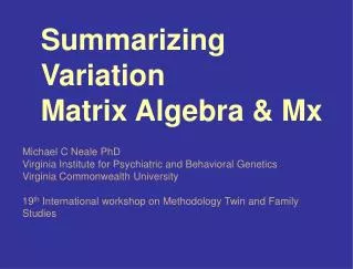
Summarizing Variation Michael C Neale PhDVirginia Institute for Psychiatric and Behavioral GeneticsVirginia Commonwealth University
Overview • Mean • Variance • Covariance • Not always necessary/desirable
Computing Mean • Formula E(xi)/N • Can compute with • Pencil • Calculator • SAS • SPSS • Mx
One Coin toss 2 outcomes Probability 0.6 0.5 0.4 0.3 0.2 0.1 0 Heads Tails Outcome
Two Coin toss 3 outcomes Probability 0.6 0.5 0.4 0.3 0.2 0.1 0 HH HT/TH TT Outcome
Four Coin toss 5 outcomes Probability 0.4 0.3 0.2 0.1 0 HHHH HHHT HHTT HTTT TTTT Outcome
Ten Coin toss 9 outcomes Probability 0.3 0.25 0.2 0.15 0.1 0.05 0 Outcome
Pascal's Triangle Probability Frequency 1 1 1 1 2 1 1 3 3 1 1 4 6 4 1 1 5 10 10 5 1 1 6 15 20 15 6 1 1 7 21 35 35 21 7 1 1/1 1/2 1/4 1/8 1/16 1/32 1/64 1/128 Pascal's friendChevalier de Mere 1654; Huygens 1657; Cardan 1501-1576
Fort Knox Toss Infinite outcomes 0.5 0.4 0.3 0.2 0.1 0 -4 -3 -2 -1 0 1 2 3 4 Heads-Tails Series 1 Gauss 1827
Variance • Measure of Spread • Easily calculated • Individual differences
Average squared deviation Normal distribution : xi di -3 -2 -1 0 1 2 3 Variance =Gdi2/N
Measuring Variation Weighs & Means • Absolute differences? • Squared differences? • Absolute cubed? • Squared squared?
Measuring Variation Ways & Means • Squared differences Fisher (1922) Squared has minimum variance under normal distribution
Covariance • Measure of association between two variables • Closely related to variance • Useful to partition variance
Deviations in two dimensions :x + + + + + + + + + + + + + + :y + + + + + + + + + + + + + + + + + + +
Deviations in two dimensions :x dx + dy :y
Measuring Covariation Area of a rectangle • A square, perimeter 4 • Area 1 1 1
Measuring Covariation Area of a rectangle • A skinny rectangle, perimeter 4 • Area .25*1.75 = .4385 .25 1.75
Measuring Covariation Area of a rectangle • Points can contribute negatively • Area -.25*1.75 = -.4385 1.75 -.25
Measuring Covariation Covariance Formula F = E(xi - :x)(yi - :y) xy (N-1)
Correlation • Standardized covariance • Lies between -1 and 1 r = F xy xy 2 2 F * F y x
Summary Formulae : = (Exi)/N Fx= E(xi - :)/(N-1) 2 2 Fxy= E(xi-:x)(yi-:y)/(N-1) r = F xy xy 2 2 F * F y x
Variance covariance matrix Several variables Var(X) Cov(X,Y) Cov(X,Z) Cov(X,Y) Var(Y) Cov(Y,Z) Cov(X,Z) Cov(Y,Z) Var(Z)
Conclusion • Means and covariances • Conceptual underpinning • Easy to compute • Can use raw data instead
Biometrical Model of QTL m - a +a d
Biometrical model for QTL Diallelic locus A/a with p as frequency of a
Classical Twin Studies Information and analysis • Summary: rmz & rdz • Basic model: A C E • rmz = A + C • rdz = .5A + C • var = A + C + E • Solve equations
Contributions to Variance Single genetic locus • Additive QTL variance • VA = 2p(1-p) [ a - d(2p-1) ]2 • Dominance QTL variance • VD= 4p2 (1-p)2 d2 • Total Genetic Variance due to locus • VQ = VA + VD
Origin of Expectations Regression model • P = aA + cC + eE • Standardize A C E • VP = a2 + c2 + e2 • Assumes A C E independent
Path analysis Elements of a path diagram • Two sorts of variable • Observed, in boxes • Latent, in circles • Two sorts of path • Causal (regression), one-headed • Correlational, two-headed
Rules of path analysis • Trace path chains between variables • Chains are traced backwards, then forwards, with one change of direction at a double headed arrow • Predicted covariance due to a chain is the product of its paths • Predicted total covariance is sum of covariance due to all possible chains
ACE model MZ twins reared together
ACE model DZ twins reared together
ACE model DZ twins reared apart
Model fitting • Takes care of replicate statistics • Maximum likelihood estimates • Confidence intervals on parameters • Overall fit of model • Comparison of nested models
Fitting models to covariance matrices • MZ covariances • 3 statistics V1 CMZ V2 • DZ covariances • 3 statistics V1 CDZ V2 • Parameters: a c e • Df = nstat - npar = 6 - 3 = 3
Model fitting to covariance matrices • Inherently compares fit to saturated model • Difference in fit between A C E model and A E model gives likelihood ratio test with df = difference in number of parameters
Confidence intervals • Two basic forms • covariance matrix of parameters • likelihood curve • Likelihood-based has some nice properties; squares of CIs on a give CI's on a2 Meeker & Escobar 1995; Neale & Miller, Behav Genet 1997
Multivariate analysis • Comorbidity • Partition into relevant components • Explicit models • One disorder or two or three • Longitudinal data analysis • Partition into new/old • Explicit models • Markov • Growth curves
Cholesky Decomposition Not a model • Provides a way to model covariance matrices • Always fits perfectly • Doesn't predict much else
Perverse Universe A E .7 .7 P NOT!
Perverse Universe A E .7 .7 .7 -.7 X Y r(X,Y)=0; Problem for almost any multivariate method
Analysis of raw data • Awesome treatment of missing values • More flexible modeling • Moderator variables • Correction for ascertainment • Modeling of means • QTL analysis
Technicolor Likelihood Function For raw data in Mx m ln Li=fi3ln [wjg(xi,:ij,Gij)] j=1 xi- vector of observed scores onn subjects :ij - vector of predicted means Gij - matrix of predicted covariances - functions of parameters
Pihat Linkage Model for Siblings Each sib pair i has different COVARIANCE
Mixture distribution model Each sib pair i has different set of WEIGHTS rQ=.0 rQ=1 rQ=.5 weightj x Likelihood under model j p(IBD=2) x P(LDL1 & LDL2 | rQ = 1 ) p(IBD=1) x P(LDL1 & LDL2 | rQ = .5 ) p(IBD=0) x P(LDL1 & LDL2 | rQ = 0 ) Total likelihood is product of weighted likelihoods
Conclusion • Model fitting has a number of advantages • Raw data can be analysed with greater flexibility • Not limited to continuous normally distributed variables
Conclusion II • Data analysis requires creative application of methods • Canned analyses are of limited use • Try to answer the question!