Download
1 / 40
400 likes | 538 Views
This chapter explores dynamic models applicable to panel data analysis. It discusses the importance of temporal aspects, particularly in forecasting and understanding variable relations. Key approaches include serial correlation models, time-varying coefficients, and the Kalman filter technique, enabling analysts to accommodate dynamic features in their models effectively. Various strategies are elaborated, including the use of lagged endogenous variables and modeling cross-sectional correlations. This comprehensive overview serves to guide practitioners in leveraging dynamic modeling techniques for enhanced analytical insight.

E N D
Chapter 8Dynamic Models • 8.1 Introduction • 8.2 Serial correlation models • 8.3 Cross-sectional correlations and time-series cross-section models • 8.4 Time-varying coefficients • 8.5 Kalman filter approach
8.1 Introduction • When is it important to consider dynamic, that is, temporal aspects of a problem? • For forecasting problems, the dynamic aspect is critical. • For other problems that are focused on understanding relations among variables, the dynamic aspects are less critical. • Still, understanding the mean and correlation structure is important for achieving efficient parameter estimators. • How does the sample size influence our choice of statistical methods? • For many panel data problems, the number of cross-sections (n) is large compared to the number of observations per subject (T ). This suggests the use of regression analysis techniques. • For other problems, T is large relative to n. This suggests borrowing from other statistical methodologies, such as multivariate time series.
Introduction – continued • How does the sample size influence the properties of our estimators? • For panel data sets where n is large compared to T, this suggests the use of asymptotic approximations where T is bounded and n tends to infinity. • In contrast, for data sets where T is large relative to n, we may achieve more reliable approximations by considering instances where • n and T approach infinity together or • where n is bounded and T tends to infinity.
Alternative approaches • There are several approaches for incorporating dynamic aspects into a panel data model. • Perhaps the easiest way is to let one of the explanatory variables be a proxy for time. • For example, we might use xij,t = t , for a linear trend in time model. • Another strategy is to analyze the differences, either through linear or proportional changes of a response. • This technique is easy to use and is natural is some areas of application. To illustrate, when examining stock prices, because of financial economics theory, we always look at proportional changes in prices, which are simply returns. • In general, one must be wary of this approach because you lose n (initial) observations when differencing.
Additional strategies • Serial Correlations • Section 8.2 expands on the discussion of the modeling dynamics through the serial correlations, introduction in Section 2.5.1. • Because of the assumption of bounded T, one need not assume stationarity of errors. • Time-varying parameters • Section 8.4 discusses problems where model parameters are allowed to vary with time. • The classic example of this is the two-way error components model, introduced in Section 3.3.2.
Additional strategies • The classic econometric method handling of dynamic aspects of a model is to include a lagged endogenous variable on the right hand side of the model. • Chapter 6 described approach, thinking of this approach as a type of Markov model. • Finally, Section 8.5 shows how to adapt the Kalman filter technique to panel data analysis. • This a flexible technique that allows analysts to incorporate time-varying parameters and broad patterns of serial correlation structures into the model. • Further, we will show how to use this technique to simultaneously model temporal and spatial patterns. • Cross-sectional correlations – Section 8.3 • When T is large relative to n, we have more opportunities to model cross-sectional correlations.
8.2 Serial correlation models • As T becomes larger, we have more opportunities to specify R = Var , the TT temporal variance-covariance matrix. • Section 2.5.1 introduced four specifications of R: (i) no correlation, (ii) compound symmetry, (iii) autoregressive of order one and (iv) unstructured. • Moving average models suggest the “Toeplitz” specification of R: • Rrs = |r-s| . This defines elements of a Toeplitz matrix. • Rrs = |r-s| for |r-s| < band and Rrs = 0 for |r-s| band. This is the banded Toeplitz matrix. • Factor analysis suggests the form R = + , • where is a matrix of unknown factor loadings and is an unknown diagonal matrix. • Useful for specifying a positive definite matrix.
Nonstationary covariance structures • With bounded T, we need not fit a stationary model to R. • A stationary AR(1) structure, it = i,t-1 + it, yields • A (nonstationary) random walk model, it = i,t-1 + it • With i0 = 0, we have Var it = t2, nonstationary
Nonstationary covariance structures • However, this is easy to invert (Exercise 4.6) and thus implement. • One can easily extend this to nonstationary AR(1) models that do not require |ρ| < 1 • use this to test for a “unit-root” • Has desirable root-n rate of asymptotics • There is a small literature on “unit-root” tests that test for stationarity as T becomes large – this is much trickier
Continuous time correlation models • When data are not equally spaced in time • consider subjects drawn from a population, yet with responses as realizations of a continuous-time stochastic process. • for each subject i, the response is {yi(t), for tR}. • Observations of the ith subject at taken at time tij so that yij = yi(tij) denotes the jth response of the ith subject • Particularly for unequally spaced data, a parametric formulation for the correlation structure is useful. • Use Rrs = Cov (ir, is) = 2( | tir – tis | ), where is the correlation function of {i(t)}. • Consider the exponential correlation model (u) = exp (– u ), for > 0 • Or the Gaussian correlation model (u) = exp (– u2 ), for > 0.
Spatially correlated models • Data may also be clustered spatially. • If there is no time element, this is straightforward. • Let dij to be some measure of spatial or geographical location of the jth observation of the ith subject. • Then, | dij – dik| is the distance between the jth and kth observations of the ith subject. • Use the correlation functions. • Could also ignore the spatial correlation for regression estimates, but use robust standard errors to account for spatial correlations.
Spatially correlated models • To account for both spatial and temporal correlation, here is a two-way model yit = i + t+ xit β + it • Stacking over i, we have where 1n is a n1 vector of ones. We re-write this as yt = α + 1nt + Xtβ + t . • Define H = Var t to be the spatial variance matrix Hij = Cov (it, jt) = 2( |di – dj | ). • Assuming that {t} is i.i.d. with variance 2, we have Var yt = Var α + 21n1n + Var t = 2 In + 2 Jn + H = 2 In + VH . • Because Cov (yr, ys) = 2 In for rs, we have V = Var y = 2 In JT + VH IT . • Use GLS from here.
8.3 Cross-sectional correlations and time-series cross-section models • When T is large relative to n, the data are sometimes referred to as time-series cross-section (TSCS) data. • Consider a TSCS model of the form yi = Xiβ + i, • we allow for correlation across different subjects through the notation Cov(i ,j ) = Vij. • Four basic specifications of cross-sectional covariancesare: • The traditional model set-up in which ols is efficient. • Heterogeneity across subjects. • Cross-sectional correlations across subjects. However, observations from different time points are uncorrelated.
Time-series cross-section models • The fourth specification is (Parks, 1967): • Cov(it, js ) = σij for t=s and i,t = ρii,t-1 + ηit . • This specification permits contemporaneous cross-correlations as well as intra-subject serial correlation through an AR(1) model. • The model has an easy to interpret cross-lag correlation function of the form, for s < t, • The drawback, particularly with specifications 3 and 4, is the number of parameters that need to be estimated in the specification of Vij.
Panel-corrected standard errors • Using OLS estimators of regression coefficients. • To account for the cross-sectional correlations, use robust standard errors. • However, now we reverse the roles of i and t. • In this context, the robust standard errors are known as panel-corrected standard errors. • Procedure for computing panel-corrected standard errors. • Calculate OLS estimators of β, bOLS, and the corresponding residuals, eit = yit – xitbOLS. • Define the estimator of the (ij)th cross-sectional covariance to be • Estimate the variance of bOLS using
8.4 Time-varying coefficients • The model is yit = z´,iti + z´,itt + x´it+ it • A matrix form is yi = Zii + Z,it + Xi+ i. • Use Ri=Var i, D=Var i and Vi= ZiDZi´+Ri • Example 1: Basic two-way model yit = i + t + x´it+ it • Example 2: Time varying coefficients model yit = x´it t+ it • Let z,it = xitand t= t - .
Forecasting • We wish to predict, or forecast, • The BLUP forecast turns out to be
Forecasting - Special Cases • No Time-Specific Components • Basic Two-Way Error Components • Baltagi (1988) and Koning (1988) (balanced) • Random Walk model
Lottery Sales Model Selection • In-sample results show that • One-way error components dominates pooled cross-sectional models • An AR(1) error specification significantly improves the fit. • The best model is probably the two-way error component model, with an AR(1) error specification
8.5 Kalman filter approach • The Kalman filter is a technique used in multivariate time series for estimating parameters from complex, recursively specified, systems. • Specifically, consider the observation equation yt = Wtδt + t and the transition equation δt = Ttδt-1 + ηt. • The approach is to consider conditional normality of yt given yt-1,…, y0, and use likelihood estimation. • The basic approach is described in Appendix D. We extend this by considering fixed and random effects, as well as allowing for spatial correlations.
Kalman filter and longitudinal data • Begin with the observation equation. yit = z,i,tαi + z,i,tλt+ xitβ + it , • The time-specific quantities are updated recursively through the transition equation, λt= 1t λt-1+ η1t. • Here, {η1t} are i.i.d mean zero random vectors. • As another way of incorporating dynamics, we also assume an AR(p) structure for the disturbances • autoregressive of order p ( AR(p) ) model i,t = 1i,t-1 +2i,t-2 + … + pi,t-p + i,t . • Here, {i,t} are i.i.d mean zero random vectors.
Transition equations • We now summarize the dynamic behavior of into a single recursive equation. • Define the p 1 vector i,t = (i,t , i,t-1, …, i,t-p+1)so that we may write • Stacking this over i=1, …, n yields • Here, t is an np 1 vector, In is an nn identity matrix and is a Kronecker (direct) product (see Appendix A.6).
Spatial correlation • The spatial correlation matrix is defined as Hn = Var(1,t, …, n,t)/2, for all t. • We assume no cross-temporal spatial correlation so that Cov(i,s, j,t )=0 for st. • Thus, • Recall that i,t = 1i,t-1 + … + pi,t-p + i,t and
Two sources of dynamic behavior • We now collect the two sources of dynamic behavior, and λ, into a single transition equation. • Assuming independence, we have • To initialize the recursion, we assume that δ0 is a vector of parameters to be estimated.
Measurement equations • For the tth time period, we have • That we express as • With • That is, fixed and random effects, with a disturbance term that is updated recursively.
Capital asset pricing model • We use the equation yit = β0i + β1ixm t + εit , • where • y is the security return in excess of the risk-free rate, • xm is the market return in excess of the risk-free rate. • We consider n = 90 firms from the insurance carriers that were listed on the CRSP files as at December 31, 1999. • The “insurance carriers” consists of those firms with standard industrial classification, SIC, codes ranging from 6310 through 6331, inclusive. • For each firm, we used sixty months of data ranging from January 1995 through December 1999.
Time-varying coefficients models • We investigate models of the form: yit = β0 + β1,i,txm,t + εit , • where εit = ρεεi,t-1 + η1,it , • and β1,i,t- β1,i = ρβ (β1,i,t-1- β1,i) + η2,it . • We assume that {εit} and {β1,i,t} are stationary AR(1) processes. • The slope coefficient, β1,i,t, is allowed to vary by both firm i and time t. • We assume that each firm has its own stationary mean β1,i and variance Var β1,i,t.
Expressing CAPM in terms of the Kalman Filter • First define jn,i to be an n 1 vector, with a “one” in the ith row and zeroes elsewhere. • Further define • Thus, with this notation, we have yit = β0 + β1,i,txmt + εit = z,i,tλt+ xitβ + it. • no random effects….
Kalman filter expressions • For the updating matrix for time-varying coefficients we use 1t= In. • AR(1) error structure, we have that p =1 and 2= . • Thus, we have • and
Table 8.5 Time-varying CAPM models • The model with both time series parameters provided the best fit. • The model without the ρε yielded a statistically significant estimate of the ρb parameters – the primary quantity of interest.
BLUPs of b1,it • Pleasant calculations show that the BLUP of 1,i,t is • where
BLUP predictors • Time series plot of BLUP predictors of the slope associated with the market returns and returns for the Lincoln National Corporation. The upper panel shows that BLUP predictor of the slopes. The lower panels shows the monthly returns.
Appendix D. State Space Model and the Kalman Filter • Basic State Space Model • Recall the observation equation yt = Wtδt + t • and the transition equation δt = Ttδt-1 + ηt. • Define • Vart-1t = Ht and Vart-1ηt = Qt. • d0 = E δ0, P0 = Var δ0 and Pt= Vartδt. • Assume that {t} and {ηt} are mutually independent. • Stacking, we have
Kalman Filter Algorithm • Taking a conditional expectation and variance of the transition equation yields the “prediction equations” dt/t-1 = Et-1δt = Ttdt-1 • and Pt/t-1 = Vart-1δt = TtPt-1Tt+ Qt. • Taking a conditional expectation and variance of measurement equation yields Et-1yt = Wt dt/t-1 • and Ft = Vart-1yt = Wt Pt/t-1 Wt+ Ht. • The updating equations are dt = dt/t-1 + Pt/t-1 WtFt-1 (yt - Wt dt/t-1) • and Pt = Pt/t-1 - Pt/t-1Wt Ft-1Wt Pt/t-1. • The updating equations are motivated by joint normality of δt and yt.
Likelihood Equations • The updating equations allows one to recursively compute Et-1yt and Ft = Vart-1yt • The likelihood of {y1, …, yT} may be expressed as • This is much simpler to evaluate (and maximize) than the full likelihood expression.
From the Kalman filter algorithm, we see that Et-1yt is a linear combination of {y1, …, yt-1 }. Thus, we may write • where L is a NN lower triangular matrix with one’s on the diagonal. • Elements of the matrix L do not depend on the random variables. • Components of Ly are mean zero and are mutually uncorrelated. • That is, conditional on {y1, …, yt-1}, the tth component of Ly, vt, has variance Ft.
Extensions • Appendix D provides extensions to the mixed linear model • The linearity of the transform turns out to be important • Section 8.5 shows how to extend this to the longitudinal data case. • We can estimate initial values as parameters • Can incorporate many different dynamic patterns for both e and l • Can also incorporate spatial relations