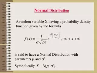
Normal distribution
Normal distribution. Learn about the properties of a normal distribution Solve problems using tables of the normal distribution Meet some other examples of continuous probability distributions. Types of variables Discrete & Continuous .

Normal distribution
E N D
Presentation Transcript
Normal distribution Learn about the properties of a normal distribution Solve problems using tables of the normal distribution Meet some other examples of continuous probability distributions
Types of variables Discrete & Continuous Describe what types of data could be described as continuous random variable X=x • Arm lengths • Eye heights
REMEMBER your box plot Middle 50% LQ UQ range
The Normal Distribution (Bell Curve) Average contents 50 Mean = μ = 50 Standard deviation = σ = 5
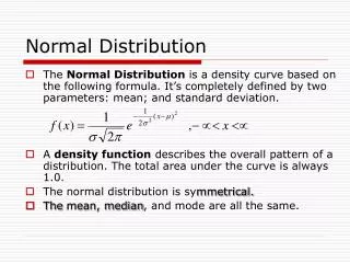
The normal distribution is a theoretical probabilitythe area under the curve adds up to one
The normal distribution is a theoretical probabilitythe area under the curve adds up to one A Normal distribution is a theoretical model of the whole population. It is perfectly symmetrical about the central value; the mean μ represented by zero.
The X axis is divided up into deviations from the mean. Below the shaded area is one deviation from the mean. As well as the mean the standard deviation (σ) must also be known.
A handy estimate – known as the Imperial Rule for a set of normal data:68% of data will fall within 1σ of the μ
Simple problems solved using the imperial rule - firstly, make a table out of the rule The heights of students at a college were found to follow a bell-shaped distribution with μ of 165cm and σ of 8 cm. What proportion of students are smaller than 157 cm 16%
Simple problems solved using the imperial rule - firstly, make a table out of the rule The heights of students at a college were found to follow a bell-shaped distribution with μ of 165cm and σ of 8 cm. Above roughly what height are the tallest 2% of the students? 165 + 2 x 8 = 181 cm
Task – class 10 minutes finish for homework • Exercise A Page 76
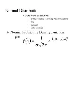
The Bell shape curve happens so when recording continuous random variables that an equation is used to model the shape exactly. Put it into your calculator and use the graph function. Sometimes you will see it using phi =.
Luckily you don’t have to use the equation each time and you don’t have to integrate it every time you need to work out the area under the curve – the normal distribution probability There are normal distribution tables
How to read the Normal distribution table Φ(z) means the area under the curve on the left of z
How to read the Normal distribution table Φ(0.24) means the area under the curve on the left of 0.24 and is this value here:
Values of Φ(z) • Φ(-1.5)=1- Φ(1.5)
Values of Φ(z) • Φ(0.8)=0.78814 (this is for the left) • Area = 1-0.78814 = 0.21186
Values of Φ(z) • Φ(1.5)=0.93319 • Φ(-1.00) =1- Φ(1.00) =1-0.84134 =0.15866 • Shaded area = Φ(1.5)- Φ(-1.00) = 0.93319 - 0.15866 = 0.77453
Task • Exercise B page 79
Solving Problems using the tables NORMAL DISTRIBUTION • The area under the curve is the probability of getting less than the z score. The total area is 1. • The tables give the probability for z-scores in the distribution X~N(0,1), that is mean =0, s.d. = 1. ALWAYS SKETCH A DIAGRAM • Read the question carefully and shade the area you want to find. If the shaded area is more than half then you can read the probability directly from the table, if it is less than half, then you need to subtract it from 1. NB If your z-score is negative then you would look up the positive from the table. The rule for the shaded area is the same as above: more than half – read from the table, less than half subtract the reading from 1.
You will have to standardise if the mean is not zero and the standard deviation is not one
Task • Exercise C page 168
Normal distribution problems in reverse • Percentage points table on page 155 • Work through examples on page 84 and do questions Exercise D on page 85
Key chapter points • The probability distribution of a continuous random variable is represented by a curve. The area under the curve in a given interval gives the probability of the value lying in that interval. • If a variable X follows a normal probability distribution, with mean μ and standard deviation σ, we write X ̴ N (μ, σ2) • The variable Z= is called the standard normal variable corresponding to X
Key chapter points cont. • If Z is a continuous random variable such that Z ̴ N (0, 1) then Φ(z)=P(Z<z) • The percentage points table shows, for probability p, the value of z such that P(Z<z)=p