Practical Path Profiling for Dynamic Optimizers
Practical Path Profiling for Dynamic Optimizers. Michael Bond, UT Austin Kathryn McKinley, UT Austin. Why path profiling?. Processors need long instruction sequences Programs have branches. A. B. C. D. E. Why path profiling?. Compiler identifies hot paths across multiple basic blocks.

Practical Path Profiling for Dynamic Optimizers
E N D
Presentation Transcript
Practical Path Profilingfor Dynamic Optimizers Michael Bond, UT Austin Kathryn McKinley, UT Austin
Why path profiling? • Processors need long instruction sequences • Programs have branches A B C D E
Why path profiling? • Compiler identifies hot paths across multiple basic blocks A B C D E
Why path profiling? • Compiler identifies hot paths across multiple basic blocks • Forms and optimizes “traces” A A B B C C D E E
Why path profiling? • Compiler identifies hot paths across multiple basic blocks • Forms and optimizes “traces” A A B B C C Oops! D E Oops! E
Why path profiling? • Compiler identifies hot paths across multiple basic blocks • Forms and optimizes “traces” Less aggressive More aggressive Hyperblocks Superblocks MSSP tasks rePLay frames Dynamo fragments
Ball-Larus path profiling Ball-Larus path profiling • Instrumentation measures execution frequency of each path • Acyclic, intraprocedural paths Targeted path profiling Edge profiling Practical path profiling
Edge profiling Ball-Larus path profiling • Hardware or sampling • Estimate hot paths from edge profile Targeted path profiling Edge profiling Practical path profiling
Ideal for dynamic optimizer Ball-Larus path profiling Targeted path profiling Edge profiling Practical path profiling
Targeted path profiling [Joshi et al. ’04] Ball-Larus path profiling • Profile-guided profiling • Accuracy good • Overhead high for dynamic optimizer Targeted path profiling Edge profiling Practical path profiling
Practical path profiling Ball-Larus path profiling Targeted path profiling Edge profiling Practical path profiling
Outline • Background • Staged dynamic optimization • Profile-guided profiling • Ball-Larus path profiling • Practical path profiling • Methodology • Edge profile-guided inlining and unrolling • Measuring accuracy with branch-flow metric • Accuracy and overhead
Staged dynamic optimization Stage 0 Static optimizations
Staged dynamic optimization Stage 0 Static optimizations Edge profile Sampling-based edge profiler
Staged dynamic optimization Stage 0 Stage 1 Static optimizations Local optimizations incl. inlining & unrolling Edge profile Sampling-based edge profiler
Staged dynamic optimization • Larger routines • Longer paths • More challenging platform for path profiling Stage 0 Stage 1 Static optimizations Local optimizations incl. inlining & unrolling Edge profile Sampling-based edge profiler
Staged dynamic optimization Stage 0 Stage 1 Static optimizations Local optimizations incl. inlining & unrolling Edge profile Path profiling instrumentation Sampling-based edge profiler
Staged dynamic optimization Stage 0 Stage 1 Static optimizations Local optimizations incl. inlining & unrolling Edge profile Path profile Path profiling instrumentation Sampling-based edge profiler
Staged dynamic optimization Stage 0 Stage 1 Stage 2 Static optimizations Local optimizations incl. inlining & unrolling Global optimizations Edge profile Path profile Path profiling instrumentation Sampling-based edge profiler
Staged dynamic optimization Edge profile: • Identifies hot and cold edges • Provides partial path profile Stage 0 Stage 1 Stage 2 Static optimizations Local optimizations incl. inlining & unrolling Global optimizations Edge profile Path profile Path profiling instrumentation Sampling-based edge profiler
Profile-guided profiling Edge profile: • Identifies hot and cold edges • Provides partial path profile Stage 0 Stage 1 Stage 2 Static optimizations Local optimizations incl. inlining & unrolling Global optimizations Edge profile Path profile Path profiling instrumentation Sampling-based edge profiler
Ball-Larus path profiling • Acyclic, intraprocedural paths • Handles cyclic routines • Instrumentation maintains execution frequency of each path • Each path computes unique integer in [0, N-1]
Ball-Larus path profiling • 4 paths [0, 3]
Ball-Larus path profiling • 4 paths [0, 3] • Each path sums to unique integer 2 0 1 0
Ball-Larus path profiling • 4 paths [0, 3] • Each path sums to unique integer Path 0 2 0 1 0
Ball-Larus path profiling • 4 paths [0, 3] • Each path sums to unique integer Path 0 Path 1 2 0 1 0
Ball-Larus path profiling • 4 paths [0, 3] • Each path sums to unique integer Path 0 Path 1 Path 2 2 0 1 0
Ball-Larus path profiling • 4 paths [0, 3] • Each path sums to unique integer Path 0 Path 1 Path 2 Path 3 2 0 1 0
Ball-Larus path profiling r=0 • r: path register • Computes path number • count: • Stores path frequencies r=r+2 r=r+1 count[r]++
Ball-Larus path profiling r=0 • r: path register • Computes path number • count: • Stores path frequencies • Array by default • Too many paths? • Hash table • High overhead r=r+2 r=r+1 count[r]++
Outline • Background • Ball-Larus path profiling • Staged dynamic optimization • Profile-guided profiling • Practical path profiling • Methodology • Edge profile-guided inlining and unrolling • Measuring accuracy with branch-flow metric • Accuracy and overhead
Practical path profiling • Goal: Reduce instrumentation overhead without hurting accuracy • Use profile-guided profiling • Strategies • Decrease number of possible paths • Avoid instrumenting paths edge profile predicts well • Simplify instrumentation on profiled paths
Practical path profiling • Goal: Reduce instrumentation overhead without hurting accuracy • Use profile-guided profiling • Strategies • Decrease number of possible paths • Avoid instrumenting paths edge profile predicts well • Simplify instrumentation on profiled paths • Techniques from targeted path profiling • Improves techniques • Adds new techniques
Strategy 1: Fewer possible paths • Goal: Hash table array • Want to remove cold paths 60 40 3 97 0 100 50 50
New Strategy 1: Fewer possible paths • Goal: Hash table array • Want to remove cold paths • Observation: A path with a cold edge is a cold path • Remove cold edges • Local and global criteria 60 40 3 97 0 100 50 50
Strategy 1: Fewer possible paths • Goal: Hash table array • Want to remove cold paths • Observation: A path with a cold edge is a cold path • Remove cold edges • Local and global criteria • Paths: 16 4
Strategy 1: Fewer possible paths • Remaining paths potentially hot • 4 paths [0, 3] 2 0 1 0
Strategy 1: Fewer possible paths r=0 • Remaining paths potentially hot • 4 paths [0, 3] r=r+2 r=r+1 count[r]++
Strategy 1: Fewer possible paths r=0 • What if cold edge taken? r=r+2 r=r+1 count[r]++
New Strategy 1: Fewer possible paths r=0 • What if cold edge taken? • Cold edges “poison” path register • Set it to N • Cold paths use [N, 2N-1] r=r+2 r=4 r=4 r=r+1 count[r]++
Strategy 1: Fewer possible paths r=0 • What if cold edge taken? • Cold edges “poison” path register • Set it to N • Cold paths use [N, 2N-1] • What if still too many possible paths? r=r+2 r=4 r=4 r=r+1 count[r]++
New Strategy 1: Fewer possible paths r=0 • What if cold edge taken? • Cold edges “poison” path register • Set it to N • Cold paths use [N, 2N-1] • What if still too many possible paths? • Adjust cold edge threshold until hashing avoided r=r+2 r=4 r=4 r=r+1 count[r]++
Strategy 2: Avoid instrumenting paths • Consider right half of CFG
Strategy 2: Avoid instrumenting paths • Consider right half of CFG • Obvious paths: Each path has an edge unique to it • Edge profile provides perfect path profile
Strategy 2: Avoid instrumenting paths • Consider right half of CFG • Obvious paths: Each path has an edge unique to it • Edge profile provides perfect path profile • We don’t instrument the right half of the CFG r=0 r=r+2 r=r+1 count[r]++
Strategy 2: Avoid instrumenting paths • Synergy: Cold edge removal creates more obvious paths
Strategy 2: Avoid instrumenting paths • Synergy: Cold edge removal creates more obvious paths • Right half is obvious
Strategy 2: Avoid instrumenting paths • What if cold edge is part of obvious and non-obvious paths?
Strategy 2: Avoid instrumenting paths • What if cold edge is part of obvious and non-obvious paths? • Right half obvious
Strategy 2: Avoid instrumenting paths r=0 • What if cold edge is part of obvious and non-obvious paths? • Right half obvious • But we haven’t avoided instrumenting it! r=r+2 r=r+1 r=4 count[r]++