Capacity Chapter 12
Capacity Chapter 12. TexPoint fonts used in EMF. Read the TexPoint manual before you delete this box.: A A A A A A A A A. Underwater Sensor Networks. Static sensor nodes plus mobile robots Dually networked optical point-to-point transmission at 300kb/s


Capacity Chapter 12
E N D
Presentation Transcript
CapacityChapter 12 TexPoint fonts used in EMF. Read the TexPoint manual before you delete this box.: AAAAAAAAA
Underwater Sensor Networks • Static sensor nodes plus mobile robots • Dually networked • optical point-to-point transmission at 300kb/s • acoustical broadcast communication at 300b/s, over hundreds of meters range. • Project AMOUR [MIT, CSIRO] • Experiments • ocean • rivers • lakes
Rating • Area maturity • Practical importance • Theory appeal First steps Text book No apps Mission critical Boooooooring Exciting
Capacity and Related Issues Protocol vs. Physical Models Capacity in Random Network Topologies Achievable Rate of Sensor Networks Scheduling Arbitrary Networks Overview
Fundamental Questions • How much communication can you have in a wireless network? • How long does it take to meet a given communication demand? • How much spatial reuse is possible? • What is the capacity of a wireless network? • Many modeling issues are connected with these questions. • You can ask these questions in many different ways that all make perfect sense, but give different answers. • In the following, we look at a few results in this context, unfortunately only superficially.
Spatial capacity is an indicator of the “data intensity” in a transmission medium. The capacity of some well-known wireless technologies IEEE 802.11b 1,000 bit/s/m² Bluetooth 30,000 bit/s/m² IEEE 802.11a 83,000 bit/s/m² Ultra-wideband 1,000,000 bit/s/m² The wireless capacity is a function of the physical layer characteristics such as available bandwidth or frequency, but also how well the protocols on top of the physical layer are implemented, in particular media access. As such capacity is a theoretical framework for MAC protocols. Motivation
Protocol Model • For lower layer protocols, a model needs to be specific about interference. A simplest interference model is an extension of the UDG. In the protocol model, a transmission by a node in at most distance 1 is received iff there is no conflicting transmission by a node in distance at most R, with R ¸ 1, sometimes just R = 2. + Easy to explain – Inherits all major drawbacks from the UDG model – Does not easily allow for designing distributed algorithms/protocols – Lots of interfering transmissions just outside the interference radius R do not sum up • Can be extended with the sameextensions as UDG, e.g. QUDG
Hop Interference (HI) • An often-used interference model is hop-interference. Here a UDG is given. Two nodes can communicate directly iff they are adjacent, and if there is no concurrent sender in the k-hop neighborhood of the receiver (in the UDG). Sometimes k = 2. • Special case of the protocol model, inheriting all its drawbacks + Simple + Allows for distributed algorithms – A node can be close but notproduce any interference (see picture) • Can be extended with the sameextensions as UDG, e.g. QUDG
Physical (SINR) Model • We look at the signal-to-noise-plus-interference (SINR) ratio. • Message arrives if SINR is larger than at receiver • Mind that the SINR model is far from perfect as well. Power level of sender u Path-loss exponent, ®= 2,...,6 Noise Minimum signal-to-interference ratio, depending on quality of hardware, etc. Distance between transmitter w and receiver v
SINR Discussion + In contrast to other low-layer models such as PM the SINR model allows for interference that does sum up. This is certainly closer to reality. However, SINR is not reality. In reality, e.g., competing transmissions may even cancel themselves, and produce less interference. In that sense the SINR model is pessimistic (interference summing up) and optimistic (if we remove the “I” from the SINR model, we have a UDG, which we know is not correct) at the same time. – SINR is “complicated”, hard to analyze – Similarly as PM, SINR does not really allow for distributed algorithms – Also, in reality, e.g. the signal fluctuates over time. Some of these issues are captured by more complicated fading channel models.
More on SINR • Often there is more than a single threshold ¯, that decides whether reception is possible or not. In many networks, a higher S/N ratio allows for more advanced modulation and coding techniques, allowing for higher throughput (e.g. Wireless LAN 802.11) • However, even more is possible: For example, assume that a receiver is receiving two signals, signal S1 being much stronger than signal S2. Then S2 has a terrible S/N ratio. However, we might be able to “subtract” the strong S1 from the total signal, and with “S – S1=S2” also get S2. • These are just two examples of how to get more than you expect.
Model Overview [Algorithmic Models for Sensor Networks, Schmid et al., 2006] • Try to proof correctness in an as “high” as possible model • For efficiency, a more optimistic (“lower”) model is fine • Lower bounds should be proved in “low” models.
Measures for Network Capacity • Throughput capacity • Number of successful packets delivered per time • Dependent on the traffic pattern • E.g.: What is the maximum achievable, over all protocols, for a random node distribution and a random destination for each source? • Transport capacity • Network transports one bit-meter when one bit has been transported a distance of one meter • Number of bit-meters transported per second • What is the maximum achievable, over all node locations, and all traffic patterns, and all protocols?
Transport Capacity • nnodes are arbitrarily located in a unit disk • We adopt the protocol model with R=2, that is a transmission is successful if and only if the sender is at least a factor 2 closer than any interfering transmitter. In other words, each node transmits with the same power, and transmissions are in synchronized slots. • What configuration and traffic pattern will yield the highest transport capacity? • Idea: Distribute n/2 senders uniformly in the unit disk. Place the n/2 receivers just close enough to senders so as to satisfy the threshold.
sender receiver Transport Capacity: Example
Transport Capacity: Understanding the example • Sender-receiver distance is £(1/√n). Assuming channel bandwidth W [bits], transport capacity is £(W√n) [bit-meter], or per node: £(W/√n) [bit-meter] • Can we do better by placing the source-destination pairs more carefully? Not really:Having a sender-receiver pair at distance dinhibits another receiver within distance upto 2d from the sender. In other words, it killsan area of £(d2). • We want to maximize n transmissions with distances d1, d2, …, dn given that the total area is less than a unit disk. This is maximized if all di = £(1/√n). So the example was asymptotically optimal. • BTW, a fun geometry problem: Given k circles with total area 1, can you always fit them in a circle with total area 2? d
More capacities… • The throughput capacity of an n node random network is • There exist constants c and c‘ such that • Transport capacity: • Per nodetransport capacity decreases with • Maximized when nodes transmit to neighbors • Throughput capacity: • For random networks, decreases with • Near-optimal when nodes transmit to neighbors • In onesentence: localcommunicationisbetter...
Even more capacities… • Similar claims hold in the physical (SINR) model as well… • Results are unchanged even if the channel can be broken into subchannels • There are literally thousands of results on capacity, e.g. • on random destinations • on power-law traffic patterns (probability to communicate to a close-by destination is higher) • communication through relays • communication in mobile networks • etc. • Problem: The model assumptions are sometimes quiteoptimistic, if not unrealistic… • Q: What is the capacity of non-random networks?
Data Gathering in Wireless Sensor Networks • Data Gathering & Aggregation • Classic application of sensor networks • Sensor nodes periodically sense environment • Relevant information needs to be transmitted to sink • Functional Capacity of Sensor Networks • Sink periodically wants to compute a function fn of sensor data • At what rate can this function be computed? (1) (2) (3) ,fn fn ,fn sink
The Simple Round-Robin Scheme • Each sensor reports its results directly to the sink (one after another). • Sink can compute one function per n rounds Achieves arate of 1/n sink x1=7 x3=4 x2=6 x4=3 (3) (2) (1) (4) fn fn fn fn x8=5 x7=9 t x5=1 x6=4 x9=2
Is there a better scheme?!? • Multi-hop relaying • In-network processing • Spatial Reuse • Pipelining • …?!? sink (1) (2) (3) (4) fn fn fn fn t
Capacity in Wireless Sensor Networks At what ratecan sensors transmit data to the sink? Scaling-laws how does rate decrease as n increases…? (1) (1/log n) (1/n) (1/√n) Only simple functions (max, min, avg,…) Answer depends on • Function to be computed • Coding techniques • Network topology • Wireless model No network coding
Practical relevance? • Efficient data gathering! • Efficient MAC layer! • This (and related) problem is studied theoretically: The Capacity of Wireless Networks Gupta, Kumar, 2000 [Arpacioglu et al, IPSN’04] [Giridhar et al, JSAC’05] [Barrenechea et al, IPSN’04] [Grossglauser et al, INFOCOM’01] [Liu et al, INFOCOM’03] [Gamal et al, INFOCOM’04] [Toumpis, TWC’03] [Kyasanur et al, MOBICOM’05] [Kodialam et al, MOBICOM’05] [Gastpar et al, INFOCOM’02] [Zhang et al, INFOCOM’05] [Mitra et al, IPSN’04] [Li et al, MOBICOM’01] [Dousse et al, INFOCOM’04] [Bansal et al, INFOCOM’03] etc… [Yi et al, MOBIHOC’03] [Perevalov et al, INFOCOM’03]
Network Topology? • Almost all capacitystudies so far makeverystrong assumptionson node deployment, topologies • randomly, uniformly distributed nodes • nodes placed on a grid • etc. What if a network looks differently…?
Capacity for Arbitrary/Worst-Case Network Topologies • What can one say about worst-case node distributions? • What can one say about arbitrary node distributions? Real Capacity How much information can be transmitted in any network? Worst-Case Capacity “Classic” Capacity How much information can be transmitted in nasty networks? How much information can be transmitted in nice networks?
Several models for wireless communication Connectivity-only models (e.g. UDG, QUDG, BIG, UBG, etc.) Interference models Protocol models Two Radii model with constant power (e.g. UDG with interference radius R=2). Nodes may use power control (transmission and interference disks of different size) Physical models SINR with constant power (every node transmitting with the same power) SINR with power control (nodes can choose power) Etc. Premise: Fundamental results should not depend on model! And indeed, classical capacity (assuming e.g. random or regular node distribution) results are similar in all the models above Are there any examples where results depend on model?! Wireless Models
Simple Example Assume a single frequency (and no fancy decoding techniques!) Let =3, =3, and N=10nW Transmission powers: PB= -15 dBm and PA= 1 dBm SINR of A at D: SINR of B at C: A sends to D, B sends to C: C D B A 4m 1m 2m NO In almost all models… Is spatial reuse possible? YES SINR w/ power control
This works in practice! [Moscibroda et al., Hotnets 2006] • Measurements using mica2 nodes • Replaced standard MAC protocol by a (tailor-made) „SINR-MAC“ • Measured for instance the following deployment... u1 u2 u3 u4 u5 u6 • Time for successfully transmitting 20,000 packets: Speed-up is almost a factor 3
Worst-Case Rate in Sensor Network: Protocol Model • Topology (worst-case!): Exponential node chain • Model: Protocol model, with power control • Assume for simplicity that the interference radius is twice the transmission radius (however, this can be relaxed easily) • Whenever a node transmits to another node all nodes to its left are in its interference range. In other words, no two nodes can transmit. • Network behaves like a single-hop network! • Same result for SINR with constant power or P ~ d®. sink xi d(sink,xi) = (1+1/)i-1 In the protocol model, the achievable rate is (1/n).
Original result was (1/log3n). [Moscibroda et al, Infocom 2006] Later improved to (1/log2n). [Moscibroda, IPSN 2007] Algorithm is centralized, complex not practical But it shows that high rates are possible even in worst-case networks Basic idea: Enable spatial reuse by exploiting SINR effects. Physical Model with Power Control In the physical model, the achievable rate is (1/polylogn), independent of the network topology.
Scheduling Algorithm – High Level Procedure • High-level idea is simple • Construct a hierarchical tree T(X) that has desirable properties 1) Initially, each node is active 2) Each node connects to closestactive node 3) Break cycles yields forest 4) Only root of each tree remains active Can be adjusted if transmission power limited loop until no active nodes Phase Scheduler: How to schedule T(X)? The resulting structure has some nice properties If each link of T(X) can be scheduled at least once in L(X) time-slots Then, a rate of 1/L(X) can be achieved
Scheduling Algorithm – Phase Scheduler • How to schedule T(X) efficiently • We need to schedule links of different magnitude simultaneously! • Only possibility: senders of small links must overpower their receiver! R(x) x d If we want to schedule both links… … R(x) must be overpowered Must transmit at power more than ~d 1) Subtle balance is needed! If senders of small links overpower their receiver… … their “safety radius” increases (spatial reuse smaller) 2)
Scheduling Algorithm – Phase Scheduler • Partition links into sets of similar length • Group sets such that links a and b in two sets in the same group have at least da¸ (c)c(a-b)¢db Each link gets a ij value Small links have large ij and vice versa Schedule links in these sets in one outer-loop iteration Intuition: Schedule links of similar length or very different length • Schedule links in a group Consider in order of decreasing length(I will not show details because of time constraints.) small large Factor 2 between two sets =1 =2 =3 Together with structure of T(x) (1/log3n) bound
Rate in Wireless Sensor Networks: Summary Worst-Case Capacity Traditional Capacity Max. rate in random, uniform deployment Max. rate in arbitrary, worst-case deployment Networks Model (1/log n) protocol model orno power control (1/n) [Giridhar, Kumar, 2005] (1/log n) physical modelwith power control (1/log2n) The Price of Worst-Case Node Placement • Exponential in protocol model • Polylogarithmicin physical model (almost no worst-case penalty!) Exponential gap between protocol and physical model!
Theoretical Implications • All MAC layer protocols we are aware of use either uniform or d power assignment. • Thus, the theoretical performance of current MAC layer protocolsis in theory as bad as scheduling every single node individually! • Faster polylogarithmic scheduling (faster MAC protocols) are theoretically possible in all (even worst-case) networks, if nodes choose their transmission power carefully. • Theoretically, there is no fundamental scaling problem with scheduling. • Theoretically efficient MAC protocols must usenon-trivial power levels! • Well, the word theory appeared in every line...
Possible Applications – Improved “Channel Capacity” • Consider a channel consisting of wireless sensor nodes • What is the throughput-capacity of this channel...? time Channel capacity is 1/3
Possible Applications – Improved “Channel Capacity” • A better strategy... • Assume node can reach 3-hop neighbor Channel capacity is 3/7 time
Possible Applications – Improved “Channel Capacity” • All such (graph-based) strategies have capacity strictly less than 1/2! • For certain and , the following strategy is better! time Channel capacity is 1/2
Possible Application – Hotspots in WLAN • Traditionally: clients assigned to (more or less) closest access point • far-terminal problem hotspots have less throughput Y X Z
Possible Application – Hotspots in WLAN • Potentially better: create hotspots with very high throughput • Every client outside a hotspot is served by one base station • Better overall throughput – increase in capacity! Y X Z
Beyond Worst-/Best-Case: Scheduling Arbitrary Links? • Given: A set of arbitrary communication requests in the plane • Each request is defined by position of source and destination • Each communication request has the same demand; if some request has a higher demand, just add links between the same sender/receiver • Just single-hop, no forwarding at intermediate nodes • Model: SINR with constant power • Goal: Minimize the time to schedule all links! • Those scheduled in the same time slot must obey SINR constraints • Example needs 3 time slots: 1,4,7 and 2,3,6 and 5,8 8 4 2 1 7 5 3 6
Some Results • Just checking whether some links can be scheduled in the same time slot is trivial. Simply test the SINR at each receiver. • In fact, even with power control this is easy. Since distances are fixed the SINR feasibility boils down to a set of linear equations: • On the other hand, scheduling all links in minimum time is difficult (NP-complete), even with constant power. [Goussevskaia et al., 2007] • With power control, thecomplexity of schedulingis still unknown. • What about approximation algorithms? Is it easy to schedule the maximum number of links in one slot? How much time do you need to deliver a given communication demand? • Some models are known, others not… N
Definition: Affectance • The „affectance“ of link lv, caused by a set of links S, is the sum of the relative interferences of the links in S on lv. This can even be scaled with noise, using an additional constant ´v. We have: with and • (We simplify by omitting noise. This gives ´v = ¯.) • A set S is SINR-feasible iff for all lv in S we have alv(S) · 1. • Affectance is additive, i.e. alv(S1) + alv(S2) = alv(S1 + S2) Interference of w on v Signal from sender v
One-Slot Scheduling with Fixed Power Levels • Given a set L={l1,…,ln} of arbitrary links, we want to maximize the number of links scheduled in one time-slot • Constant approximation algorithm: • Input: L; Output: S; • Repeat • Add shortest link lv in L to S; • Delete all lw in L, where dwv≤c¢dvv; • Delete all lw in L, where aS(lw) ≥ 2/3; • Until L=ø; • Return S; • *Affectedness has a similar definition as affectance; it also tells how much interference a link can tolerate, i.e. aS(lv) = 1 if SINRS(lv) = β Schedule “strong” links first Constant c>2, c=f(α,β) Links with receivers sw too close to sender rv Links with high affectedness* Set of links S is valid iff aS(lv) ≤1 foralllv in S
R2 R1 ± rv ± One-Slot Scheduling: Correctness Proof • We need to prove affectedness aS(lv) ≤1 for all lv in S • All senders in set Sv+ have pair wise distance ± = (c-1)dvv. • We partition the space in infinitely many rings of thickness ±. • There is no sender in Sv+ in circle R0 • A sender in ring Rk has at least distance k± • The number of senders in ring Rk is O(k) • Affectedness from ring Rk is O(¯k1-®±-®) • Total affectedness is O(§k¸1¯k1-®±-®) · 1/3, for ® > 2 and large enough constant c = f(α,β) Sv+:set of longer (≥) links in S, i.e., added afterlv Sv-:set of shorter (≤) links in S, i.e., added before lv aSv+(lv) ≤1/3 (? See below!) aSv-(lv) ≤2/3 (OK! by algo) Rk …
rv cdvv One-SlotScheduling: Approximation Proof • Count the number of links deleted by ALG that could have been scheduled in the optimum solution OPT: OPT’ = OPT \ ALG • Claim 1: |OPT1|≤ ½1|ALG|, with ½1 = f(c) • Proof: Ifthe optimal wants to schedulemorethan½1 links aroundreceiverrv, thentwo of these links have to beveryclose, and would not satisfythe SINR condition (sincetheirlengthis at leastthelength of link lv). OPT’ = OPT1 + OPT2 OPT1: links deleted in step 1 OPT2: links deleted in step 2
Consider two disjoint sets B and R of blue and red points in the plane. If |B| > 5q|R| then at least one point b in B is q-blue-dominant. Definition: a point b in B is q-blue-dominant (q in Z+) if, for every ball of radius d around b, there are q times more blue than red points. Proof: for each red point r in R, remove q “guarding sets” of r, i.e., q times the 5 closest blue points in all directions. After processing all the red points, at least one blue point b* is left, since |B| > 5q|R|. Point b* is blue-dominant, since all red points in R are “guarded” by at least q blue points from all directions. Helper Lemma: Blue-Dominant Centers Lemma
One-SlotScheduling: Approximation Proof (Part 2) • Claim 2: |OPT2|≤ ½2|ALG|, ½2=10 • Proof: Let B = OPT2 (senders) and R = ALG (senders also) • Assume for the sake of contradiction that |B|>10|R|. • By the blue dominant centers lemma, there is a 2-blue-dominant point b in OPT2. Since b is 2-blue-dominant, it is twice as much affected by OPT2 than by ALG. (Really, it is the receiver of link lb that is affected but thanks to the clearing of the neighborhood, the receiver is “close” to the sender; some nasty details omitted). • In other words, we have aALG(lb) < ½¢aOPT2(lb). With aOPT2(lb) ≤ 1 we have aALG(lb) < ½. This contradicts that link lbhas beendeletedbystep 2 of thealgorithm, sincestep 2 onlydeletes links withaS(lb) ≥ 2/3. • In summary, (½1+½2)¢|ALG|¸|OPT1| + |OPT2| = |OPT’| = |OPT \ ALG| ¸ |OPT| – |ALG|. That is, |ALG| ¸|OPT| /(½1+½2+1) = (|OPT|).
SINR Robustness • Given a set of scheduling requests S. We can schedule the set in T time, iff we can partition the set in T SINR-feasible subsets S1,…, ST • What happens if we change the parameters a bit, e.g. what if we now need to deal with a different ¯? Can it be that changing ¯ by some constant factor will lead to a totally different solution? • In general, what if the world is not perfect?! • What if antennas are not perfectly omnidirectional? • What if signals are not perfectly summing up? • What if signal-to-noise ratio is not perfectly equal to ¯? • Luckily the SINR model is robust against minor (constant) changes
General Robustness Algorithm • A set S is SINRÁ-feasible iff for all lv in S we have alv(S) ·Á. A schedule is SINRÁ-feasible if all its slots are SINRÁ-feasible. • This generalized feasibility essentially covers all model changes • From a SINR-feasible schedule to a SINRÁ-feasible schedule: • For each slot S in a SINR-feasible schedule, process links of S in decreasing order of their length, i.e., l1, l2, …, lk2S, with lv¸lv+1. For each link lv, assign lv to Sj with minimum j with alv(Sj) ·Á/2.Then, the affectance on lvby longer links is at most Á/2.By additivity of affectance, the number of sets is at most d2/Áe. • For each set Sj, do the process in reverse order (short links first), getting sets Sj1, Sj2, …, Sjk. Now, the affectance on lvby shorter links is at most Á/2. Thus, the total affectance is at most Á for each link. Also each original set S is partitioned into at most d2/Áe2 sets.