Download
1 / 54
540 likes | 699 Views
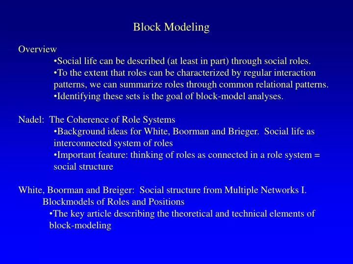
Block Modeling. Overview Social life can be described (at least in part) through social roles. To the extent that roles can be characterized by regular interaction patterns, we can summarize roles through common relational patterns. Identifying these sets is the goal of block-model analyses.

E N D
Block Modeling • Overview • Social life can be described (at least in part) through social roles. • To the extent that roles can be characterized by regular interaction patterns, we can summarize roles through common relational patterns. • Identifying these sets is the goal of block-model analyses. • Nadel: The Coherence of Role Systems • Background ideas for White, Boorman and Brieger. Social life as interconnected system of roles • Important feature: thinking of roles as connected in a role system = social structure • White, Boorman and Breiger: Social structure from Multiple Networks I. Blockmodels of Roles and Positions • The key article describing the theoretical and technical elements of block-modeling
Nadel: The Coherence of Role Systems • Elements of a Role: • Rights and obligations with respect to other people or classes of people • Roles require a ‘role compliment’ another person who the role-occupant acts with respect to • Examples: • Parent - child, Teacher - student, Lover - lover, Friend - Friend, Husband - Wife, etc. • Nadel (Following functional anthropologists and sociologists) defines ‘logical’ types of roles, and then examines how they can be linked together.
Nadel: The Coherence of Role Systems Nadel describes role patterns in the book. In the chapter we read, he focuses on how these various roles fit together to form a coherent whole. Roles are collected in people through the ‘summation of roles” Necessary: Some roles fit together necessarily. For example, the expected interaction patterns of “son-in-law” are implied through the joint roles of “Husband” and “Spouse-Parent” Coincidental: Some roles tend to go together empirically, but they need not (businessman & club member, for example). Distinguishing the two is a matter of usefulness and judgement, but relates to social substitutability. The distinction reverts to how the system as a whole will be held together in the face of changes in role occupants.
Nadel: The Coherence of Role Systems Given that roles can be identified as ‘going together’ is there a logic that underlies their connection? Nadel uses a functional description based on ascription and achievement:
Nadel: The Coherence of Role Systems And he gives an example of a simple role system: Nadel’s task is to make sense of these roles, to identify how they are interconnected to form a system -- a coherent structure. This is a difficult task to do analytically, as the eventual failure of Parsonian functionalism shows.
White et al: From logical role systems to empirical social structures With the fall of parsons and functionalism in the late 60s, many of the ideas about social structure and system were also tossed. White et al demonstrate how we can understand social structure as the intercalation of roles, without the a priori logical categories. Start with some basic ideas of what a role is: An exchange of something (support, ideas, commands, etc) between actors. Thus, we might represent a family as:
Romantic Love Bickers with White et al: From logical role systems to empirical social structures Start with some basic ideas of what a role is: An exchange of something (support, ideas, commands, etc) between actors. Thus, we might represent a family as: H W C C C Provides food for (and there are, of course, many other relations inside the family)
White et al: From logical role systems to empirical social structures The key idea, is that we can express a role through a relation (or set of relations) and thus a social system by the inventory of roles. If roles equate to positions in an exchange system, then we need only identify particular aspects of a position. But what aspect? Structural Equivalence Two actors are structurally equivalent if they have the same types of ties to the same people.
Structural Equivalence A single relation
Structural Equivalence Graph reduced to positions
Alternative notions of equivalence Instead of exact same ties to exact same alters, you look for nodes with similar ties to similar types of alters
Blockmodeling: basic steps In any positional analysis, there are 4 basic steps: 1) Identify a definition of equivalence 2) Measure the degree to which pairs of actors are equivalent 3) Develop a representation of the equivalencies 4) Assess the adequacy of the representation
1) Identify a definition of equivalence • Structural Equivalence: • Two actors are equivalent if they have the same type of ties to the same people.
1) Identify a definition of equivalence Automorphic Equivalence: Actors occupy indistinguishable structural locations in the network. That is, that they are in isomorphic positions in the network. Two graphs are isomorphic if there is some mapping of nodes to positions that equates the two. For example, all 030T triads are isomorphic. A graph is automorphic, if there are patterns internal to the graph that are equated (if the mapping goes from the set of nodes in the graph to other nodes in the graph). In general, automorphically equivalent nodes are equivalent with respect to all graph theoretic properties (I.e. degree, number of people reachable, centrality, etc.)
1) Identify a definition of equivalence Regular Equivalence: Regular equivalence does not require actors to have identical ties to identical actors or to be structurally indistinguishable. Actors who are regularly equivalent have identical ties to and from equivalent actors. If actors i and j are regularly equivalent, then for all relations and for all actors, if i k, then there exists some actor l such that j l and k is regularly equivalent to l.
Regular Equivalence: There may be multiple regular equivalence partitions in a network, and thus we tend to want to find the maximal regular equivalence position, the one with the fewest positions.
Role or Local Equivalence: While most equivalence measures focus on position within the full network, some measures focus only on the patters within the local tie neighborhood. These have been called ‘local role’ equivalence. In the example we’ve been using, they revert to automorphic equivalence • Note that: • Structurally equivalent actors are automorphically equivalent, • Automorphically equivalent actors are regularly equivalent. • Structurally equivalent and automorphically equivalent actors are role equivalent • In practice, we tend to ignore some of these fine distinctions, as they get blurred quickly once we have to operationalize them in real graphs. It turns out that few people are ever exactly equivalent, and thus we approximate the links between the types. • In all cases, the procedure can work over multiple relations simultaneously. • The process of identifying positions is called blockmodeling, and requires identifying a measure of similarity among nodes.
Blockmodeling is the process of identifying these types of positions. A block is a section of the adjacency matrix - a “group” of people. 0 1 1 1 0 0 0 0 0 0 0 0 0 0 1 0 0 0 1 1 0 0 0 0 0 0 0 0 1 0 0 1 0 0 1 1 1 1 0 0 0 0 1 0 1 0 0 0 1 1 1 1 0 0 0 0 0 1 0 0 0 1 0 0 0 0 1 1 1 1 0 1 0 0 1 0 0 0 0 0 1 1 1 1 0 0 1 1 0 0 0 0 0 0 0 0 0 0 0 0 1 1 0 0 0 0 0 0 0 0 0 0 0 0 1 1 0 0 0 0 0 0 0 0 0 0 0 0 1 1 0 0 0 0 0 0 0 0 0 0 0 0 0 0 1 1 0 0 0 0 0 0 0 0 0 0 0 0 1 1 0 0 0 0 0 0 0 0 0 0 0 0 1 1 0 0 0 0 0 0 0 0 0 0 0 0 1 1 0 0 0 0 0 0 0 0 Here I have blocked structurally equivalent actors
Once you block the matrix, reduce it, based on the number of ties in the cell of interest. The key values are a zero block (no ties) and a one-block (all ties present): 1 2 3 4 5 6 1 0 1 1 0 0 0 2 1 0 0 1 0 0 3 1 0 1 0 1 0 4 0 1 0 1 0 1 5 0 0 1 0 0 0 6 0 0 0 1 0 0 1 2 3 4 5 6 1 . 1 1 1 0 0 0 0 0 0 0 0 0 0 1 . 0 0 1 1 0 0 0 0 0 0 0 0 1 0 . 1 0 0 1 1 1 1 0 0 0 0 1 0 1 . 0 0 1 1 1 1 0 0 0 0 0 1 0 0 . 1 0 0 0 0 1 1 1 1 0 1 0 0 1 . 0 0 0 0 1 1 1 1 0 0 1 1 0 0 . 0 0 0 0 0 0 0 0 0 1 1 0 0 0 . 0 0 0 0 0 0 0 0 1 1 0 0 0 0 . 0 0 0 0 0 0 0 1 1 0 0 0 0 0 . 0 0 0 0 0 0 0 0 1 1 0 0 0 0 . 0 0 0 0 0 0 0 1 1 0 0 0 0 0 . 0 0 0 0 0 0 1 1 0 0 0 0 0 0 . 0 0 0 0 0 1 1 0 0 0 0 0 0 0 . 2 3 4 5 6 Structural equivalence thus generates 6 positions in the network
Once you partition the matrix, reduce it: . 1 1 1 0 0 0 0 0 0 0 0 0 0 1 . 0 0 1 1 0 0 0 0 0 0 0 0 1 0 . 1 0 0 1 1 1 1 0 0 0 0 1 0 1 . 0 0 1 1 1 1 0 0 0 0 0 1 0 0 . 1 0 0 0 0 1 1 1 1 0 1 0 0 1 . 0 0 0 0 1 1 1 1 0 0 1 1 0 0 . 0 0 0 0 0 0 0 0 0 1 1 0 0 0 . 0 0 0 0 0 0 0 0 1 1 0 0 0 0 . 0 0 0 0 0 0 0 1 1 0 0 0 0 0 . 0 0 0 0 0 0 0 0 1 1 0 0 0 0 . 0 0 0 0 0 0 0 1 1 0 0 0 0 0 . 0 0 0 0 0 0 1 1 0 0 0 0 0 0 . 0 0 0 0 0 1 1 0 0 0 0 0 0 0 . 1 2 3 1 1 1 0 2 1 1 1 3 0 1 0 1 2 3 Regular equivalence (here I placed a one in the image matrix if there were any ties in the ij block)
To get a block model, you have to measure the similarity between each pair. If two actors are structurally equivalent, then they will have exactly similar patterns of ties to other people. Consider the example again: C and D match on 12 other people 1 2 3 4 5 6 C D Match 11 1 00 1 . 1 0 1 . 0 00 1 00 1 11 1 11 1 11 1 11 1 00 1 00 1 00 1 00 1 Sum: 12 1 . 1 1 1 0 0 0 0 0 0 0 0 0 0 1 . 0 0 1 1 0 0 0 0 0 0 0 0 1 0 . 1 0 0 1 1 1 1 0 0 0 0 1 0 1 . 0 0 1 1 1 1 0 0 0 0 0 1 0 0 . 1 0 0 0 0 1 1 1 1 0 1 0 0 1 . 0 0 0 0 1 1 1 1 0 0 1 1 0 0 . 0 0 0 0 0 0 0 0 0 1 1 0 0 0 . 0 0 0 0 0 0 0 0 1 1 0 0 0 0 . 0 0 0 0 0 0 0 1 1 0 0 0 0 0 . 0 0 0 0 0 0 0 0 1 1 0 0 0 0 . 0 0 0 0 0 0 0 1 1 0 0 0 0 0 . 0 0 0 0 0 0 1 1 0 0 0 0 0 0 . 0 0 0 0 0 1 1 0 0 0 0 0 0 0 . 2 3 4 5 6
If the model is going to be based on asymmetric or multiple relations, you simply stack the various relations: Stacked Romance 0 1 0 0 0 1 0 0 0 0 0 0 0 0 0 0 0 0 0 0 0 0 0 0 0 0 1 0 0 0 1 0 0 0 0 0 0 0 0 0 0 0 0 0 0 0 0 0 0 0 H W 0 0 1 1 1 0 0 1 1 1 0 0 0 0 0 0 0 0 0 0 0 0 0 0 0 Feeds 0 0 1 1 1 0 0 1 1 1 0 0 0 0 0 0 0 0 0 0 0 0 0 0 0 C C C 0 0 0 0 0 0 0 0 0 0 1 1 0 0 0 1 1 0 0 0 1 1 0 0 0 Romantic Love Provides food for Bicker 0 0 0 0 0 0 0 0 0 0 0 0 0 1 1 0 0 1 0 0 0 0 1 1 0 Bickers with 0 0 0 0 0 0 0 0 0 0 0 0 0 1 1 0 0 1 0 1 0 0 1 1 0
For the entire matrix, we get: 0 8 7 7 5 5 11 11 11 11 7 7 7 7 8 0 5 5 7 7 7 7 7 7 11 11 11 11 7 5 0 12 0 0 8 8 8 8 4 4 4 4 7 5 12 0 0 0 8 8 8 8 4 4 4 4 5 7 0 0 0 12 4 4 4 4 8 8 8 8 5 7 0 0 12 0 4 4 4 4 8 8 8 8 11 7 8 8 4 4 0 12 12 12 8 8 8 8 11 7 8 8 4 4 12 0 12 12 8 8 8 8 11 7 8 8 4 4 12 12 0 12 8 8 8 8 11 7 8 8 4 4 12 12 12 0 8 8 8 8 7 11 4 4 8 8 8 8 8 8 0 12 12 12 7 11 4 4 8 8 8 8 8 8 12 0 12 12 7 11 4 4 8 8 8 8 8 8 12 12 0 12 7 11 4 4 8 8 8 8 8 8 12 12 12 0 (number of agreements for each ij pair)
The metric used to measure structural equivalence by White, Boorman and Brieger is the correlation between each node’s set of ties. For the example, this would be: 1.00 -0.20 0.08 0.08 -0.19 -0.19 0.77 0.77 0.77 0.77 -0.26 -0.26 -0.26 -0.26 -0.20 1.00 -0.19 -0.19 0.08 0.08 -0.26 -0.26 -0.26 -0.26 0.77 0.77 0.77 0.77 0.08 -0.19 1.00 1.00 -1.00 -1.00 0.36 0.36 0.36 0.36 -0.45 -0.45 -0.45 -0.45 0.08 -0.19 1.00 1.00 -1.00 -1.00 0.36 0.36 0.36 0.36 -0.45 -0.45 -0.45 -0.45 -0.19 0.08 -1.00 -1.00 1.00 1.00 -0.45 -0.45 -0.45 -0.45 0.36 0.36 0.36 0.36 -0.19 0.08 -1.00 -1.00 1.00 1.00 -0.45 -0.45 -0.45 -0.45 0.36 0.36 0.36 0.36 0.77 -0.26 0.36 0.36 -0.45 -0.45 1.00 1.00 1.00 1.00 -0.20 -0.20 -0.20 -0.20 0.77 -0.26 0.36 0.36 -0.45 -0.45 1.00 1.00 1.00 1.00 -0.20 -0.20 -0.20 -0.20 0.77 -0.26 0.36 0.36 -0.45 -0.45 1.00 1.00 1.00 1.00 -0.20 -0.20 -0.20 -0.20 0.77 -0.26 0.36 0.36 -0.45 -0.45 1.00 1.00 1.00 1.00 -0.20 -0.20 -0.20 -0.20 -0.26 0.77 -0.45 -0.45 0.36 0.36 -0.20 -0.20 -0.20 -0.20 1.00 1.00 1.00 1.00 -0.26 0.77 -0.45 -0.45 0.36 0.36 -0.20 -0.20 -0.20 -0.20 1.00 1.00 1.00 1.00 -0.26 0.77 -0.45 -0.45 0.36 0.36 -0.20 -0.20 -0.20 -0.20 1.00 1.00 1.00 1.00 -0.26 0.77 -0.45 -0.45 0.36 0.36 -0.20 -0.20 -0.20 -0.20 1.00 1.00 1.00 1.00 Another common metric is the Euclidean distance between pairs of actors, which you then use in a standard cluster analysis.
The initial method for finding structurally equivalent positions was CONCOR, the CONvergence of iterated CORrelations. Concor iteration 1: 1.00 -.77 0.55 0.55 -.57 -.57 0.95 0.95 0.95 0.95 -.75 -.75 -.75 -.75 -.77 1.00 -.57 -.57 0.55 0.55 -.75 -.75 -.75 -.75 0.95 0.95 0.95 0.95 0.55 -.57 1.00 1.00 -1.0 -1.0 0.73 0.73 0.73 0.73 -.75 -.75 -.75 -.75 0.55 -.57 1.00 1.00 -1.0 -1.0 0.73 0.73 0.73 0.73 -.75 -.75 -.75 -.75 -.57 0.55 -1.0 -1.0 1.00 1.00 -.75 -.75 -.75 -.75 0.73 0.73 0.73 0.73 -.57 0.55 -1.0 -1.0 1.00 1.00 -.75 -.75 -.75 -.75 0.73 0.73 0.73 0.73 0.95 -.75 0.73 0.73 -.75 -.75 1.00 1.00 1.00 1.00 -.77 -.77 -.77 -.77 0.95 -.75 0.73 0.73 -.75 -.75 1.00 1.00 1.00 1.00 -.77 -.77 -.77 -.77 0.95 -.75 0.73 0.73 -.75 -.75 1.00 1.00 1.00 1.00 -.77 -.77 -.77 -.77 0.95 -.75 0.73 0.73 -.75 -.75 1.00 1.00 1.00 1.00 -.77 -.77 -.77 -.77 -.75 0.95 -.75 -.75 0.73 0.73 -.77 -.77 -.77 -.77 1.00 1.00 1.00 1.00 -.75 0.95 -.75 -.75 0.73 0.73 -.77 -.77 -.77 -.77 1.00 1.00 1.00 1.00 -.75 0.95 -.75 -.75 0.73 0.73 -.77 -.77 -.77 -.77 1.00 1.00 1.00 1.00 -.75 0.95 -.75 -.75 0.73 0.73 -.77 -.77 -.77 -.77 1.00 1.00 1.00 1.00
The initial method for finding structurally equivalent positions was CONCOR, the CONvergence of iterated CORrelations. Concor iteration 2: 1.00 -.99 0.94 0.94 -.94 -.94 0.99 0.99 0.99 0.99 -.99 -.99 -.99 -.99 -.99 1.00 -.94 -.94 0.94 0.94 -.99 -.99 -.99 -.99 0.99 0.99 0.99 0.99 0.94 -.94 1.00 1.00 -1.0 -1.0 0.97 0.97 0.97 0.97 -.97 -.97 -.97 -.97 0.94 -.94 1.00 1.00 -1.0 -1.0 0.97 0.97 0.97 0.97 -.97 -.97 -.97 -.97 -.94 0.94 -1.0 -1.0 1.00 1.00 -.97 -.97 -.97 -.97 0.97 0.97 0.97 0.97 -.94 0.94 -1.0 -1.0 1.00 1.00 -.97 -.97 -.97 -.97 0.97 0.97 0.97 0.97 0.99 -.99 0.97 0.97 -.97 -.97 1.00 1.00 1.00 1.00 -.99 -.99 -.99 -.99 0.99 -.99 0.97 0.97 -.97 -.97 1.00 1.00 1.00 1.00 -.99 -.99 -.99 -.99 0.99 -.99 0.97 0.97 -.97 -.97 1.00 1.00 1.00 1.00 -.99 -.99 -.99 -.99 0.99 -.99 0.97 0.97 -.97 -.97 1.00 1.00 1.00 1.00 -.99 -.99 -.99 -.99 -.99 0.99 -.97 -.97 0.97 0.97 -.99 -.99 -.99 -.99 1.00 1.00 1.00 1.00 -.99 0.99 -.97 -.97 0.97 0.97 -.99 -.99 -.99 -.99 1.00 1.00 1.00 1.00 -.99 0.99 -.97 -.97 0.97 0.97 -.99 -.99 -.99 -.99 1.00 1.00 1.00 1.00 -.99 0.99 -.97 -.97 0.97 0.97 -.99 -.99 -.99 -.99 1.00 1.00 1.00 1.00
The initial method for finding structurally equivalent positions was CONCOR, the CONvergence of iterated CORrelations. Concor iteration 3: 1.00 -1.0 1.00 1.00 -1.0 -1.0 1.00 1.00 1.00 1.00 -1.0 -1.0 -1.0 -1.0 -1.0 1.00 -1.0 -1.0 1.00 1.00 -1.0 -1.0 -1.0 -1.0 1.00 1.00 1.00 1.00 1.00 -1.0 1.00 1.00 -1.0 -1.0 1.00 1.00 1.00 1.00 -1.0 -1.0 -1.0 -1.0 1.00 -1.0 1.00 1.00 -1.0 -1.0 1.00 1.00 1.00 1.00 -1.0 -1.0 -1.0 -1.0 -1.0 1.00 -1.0 -1.0 1.00 1.00 -1.0 -1.0 -1.0 -1.0 1.00 1.00 1.00 1.00 -1.0 1.00 -1.0 -1.0 1.00 1.00 -1.0 -1.0 -1.0 -1.0 1.00 1.00 1.00 1.00 1.00 -1.0 1.00 1.00 -1.0 -1.0 1.00 1.00 1.00 1.00 -1.0 -1.0 -1.0 -1.0 1.00 -1.0 1.00 1.00 -1.0 -1.0 1.00 1.00 1.00 1.00 -1.0 -1.0 -1.0 -1.0 1.00 -1.0 1.00 1.00 -1.0 -1.0 1.00 1.00 1.00 1.00 -1.0 -1.0 -1.0 -1.0 1.00 -1.0 1.00 1.00 -1.0 -1.0 1.00 1.00 1.00 1.00 -1.0 -1.0 -1.0 -1.0 -1.0 1.00 -1.0 -1.0 1.00 1.00 -1.0 -1.0 -1.0 -1.0 1.00 1.00 1.00 1.00 -1.0 1.00 -1.0 -1.0 1.00 1.00 -1.0 -1.0 -1.0 -1.0 1.00 1.00 1.00 1.00 -1.0 1.00 -1.0 -1.0 1.00 1.00 -1.0 -1.0 -1.0 -1.0 1.00 1.00 1.00 1.00 -1.0 1.00 -1.0 -1.0 1.00 1.00 -1.0 -1.0 -1.0 -1.0 1.00 1.00 1.00 1.00
The initial method for finding structurally equivalent positions was CONCOR, the CONvergence of iterated CORrelations. Concor iteration 3: 1.00 1.00 1.00 1.00 1.00 1.00 1.00 -1.0 -1.0 -1.0 -1.0 -1.0 -1.0 -1.0 1.00 1.00 1.00 1.00 1.00 1.00 1.00 -1.0 -1.0 -1.0 -1.0 -1.0 -1.0 -1.0 1.00 1.00 1.00 1.00 1.00 1.00 1.00 -1.0 -1.0 -1.0 -1.0 -1.0 -1.0 -1.0 1.00 1.00 1.00 1.00 1.00 1.00 1.00 -1.0 -1.0 -1.0 -1.0 -1.0 -1.0 -1.0 1.00 1.00 1.00 1.00 1.00 1.00 1.00 -1.0 -1.0 -1.0 -1.0 -1.0 -1.0 -1.0 1.00 1.00 1.00 1.00 1.00 1.00 1.00 -1.0 -1.0 -1.0 -1.0 -1.0 -1.0 -1.0 1.00 1.00 1.00 1.00 1.00 1.00 1.00 -1.0 -1.0 -1.0 -1.0 -1.0 -1.0 -1.0 -1.0 -1.0 -1.0 -1.0 -1.0 -1.0 -1.0 1.00 1.00 1.00 1.00 1.00 1.00 1.00 -1.0 -1.0 -1.0 -1.0 -1.0 -1.0 -1.0 1.00 1.00 1.00 1.00 1.00 1.00 1.00 -1.0 -1.0 -1.0 -1.0 -1.0 -1.0 -1.0 1.00 1.00 1.00 1.00 1.00 1.00 1.00 -1.0 -1.0 -1.0 -1.0 -1.0 -1.0 -1.0 1.00 1.00 1.00 1.00 1.00 1.00 1.00 -1.0 -1.0 -1.0 -1.0 -1.0 -1.0 -1.0 1.00 1.00 1.00 1.00 1.00 1.00 1.00 -1.0 -1.0 -1.0 -1.0 -1.0 -1.0 -1.0 1.00 1.00 1.00 1.00 1.00 1.00 1.00 -1.0 -1.0 -1.0 -1.0 -1.0 -1.0 -1.0 1.00 1.00 1.00 1.00 1.00 1.00 1.00 1 3 4 7 8 9 10 2 5 6 11 12 13 14
Repeat the process on the resulting 1-blocks until you have reached structural equivalent blocks Because CONCOR splits every sub-group into two groups, you get a partition tree that looks something like this:
Automorphic and Regular equivalence are more difficult to find, and require iteratively searching over possible class assignments for sets that have the same graph theoretic patterns. Usually start with a set of nodes defined as similar on a number of network measures, then look within these classes for automorphic equivalence classes. A theoretically appealing method for finding structures that are very similar to regular equivalence, role equivalence, uses the triad census. Each node is involved in (n-1)(n-2)/2 triads, and occupies a particular position in each of these triads. These positions are summarized in the following figure:
Triadic Position Census: 36 Positions within 16 Directed Triads 120D_S 003 021C_S 120D_E 021C_B 012_S 021C_E 120U_S 012_E 120U_E 111D_S 012_I 120C_S 111D_B 102_D 120C_B 111D_E 102_I 030T_S 120C_E 111U_S 030T_B 021D_S 210_S 111U_B 030T_E 021D_E 210_B 111U_E 021U_S 210_B 030C 021U_E 201_S 300 201_B Indicates the position.
Triadic Position Census: 40 Positions within all mutual ties but two types of relations
36 36 10 10 10 10 43 43 43 43 43 43 43 43 0 0 0 0 0 0 0 0 0 0 0 0 0 0 0 0 0 0 0 0 0 0 0 0 0 0 0 0 0 0 0 0 0 0 0 0 0 0 0 0 0 0 20 20 41 41 41 41 14 14 14 14 14 14 14 14 9 9 11 11 11 11 12 12 12 12 12 12 12 12 0 0 0 0 0 0 0 0 0 0 0 0 0 0 0 0 0 0 0 0 0 0 0 0 0 0 0 0 0 0 0 0 0 0 0 0 0 0 0 0 0 0 0 0 0 0 0 0 0 0 0 0 0 0 0 0 0 0 0 0 0 0 0 0 0 0 0 0 0 0 0 0 0 0 0 0 0 0 0 0 0 0 0 0 0 0 0 0 0 0 0 0 0 0 0 0 0 0 0 0 0 0 0 0 0 0 0 0 0 0 0 0 0 0 0 0 0 0 0 0 0 0 0 0 0 0 0 0 0 0 0 0 0 0 0 0 0 0 0 0 0 0 0 0 0 0 0 0 0 0 0 0 0 0 0 0 0 0 0 0 0 0 0 0 0 0 0 0 0 0 0 0 0 0 0 0 0 0 0 0 0 0 0 0 0 0 0 0 0 0 0 0 0 0 0 0 0 0 0 0 0 0 0 0 0 0 0 0 0 0 0 0 0 0 0 0 0 0 0 0 0 0 0 0 0 0 0 0 0 0 0 0 0 0 0 0 0 0 10 10 1 1 1 1 8 8 8 8 8 8 8 8 2 2 10 10 10 10 0 0 0 0 0 0 0 0 0 0 0 0 0 0 0 0 0 0 0 0 0 0 0 0 0 0 0 0 0 0 0 0 0 0 0 0 0 0 0 0 0 0 0 0 0 0 0 0 0 0 0 0 0 0 0 0 0 0 0 0 0 0 0 0 0 0 0 0 0 0 0 0 0 0 0 0 0 0 0 0 0 0 0 0 0 0 0 0 0 0 0 0 0 0 0 0 0 0 0 0 0 0 0 0 0 0 0 0 0 0 0 0 0 0 0 0 0 0 0 0 0 0 0 0 0 0 0 0 0 0 0 0 0 0 0 0 0 0 0 0 0 0 0 0 0 0 0 0 1 1 5 5 5 5 1 1 1 1 1 1 1 1 Triad position vectors for the example network, resulting in 3 positions:
Correlating each person’s triad position vector with each other persons results in the following table, which clearly shows the positions that are equivalent: 1.00 1.00 0.64 0.64 0.64 0.64 0.98 0.98 0.98 0.98 0.98 0.98 0.98 0.98 1.00 1.00 0.64 0.64 0.64 0.64 0.98 0.98 0.98 0.98 0.98 0.98 0.98 0.98 0.64 0.64 1.00 1.00 1.00 1.00 0.50 0.50 0.50 0.50 0.50 0.50 0.50 0.50 0.64 0.64 1.00 1.00 1.00 1.00 0.50 0.50 0.50 0.50 0.50 0.50 0.50 0.50 0.64 0.64 1.00 1.00 1.00 1.00 0.50 0.50 0.50 0.50 0.50 0.50 0.50 0.50 0.64 0.64 1.00 1.00 1.00 1.00 0.50 0.50 0.50 0.50 0.50 0.50 0.50 0.50 0.98 0.98 0.50 0.50 0.50 0.50 1.00 1.00 1.00 1.00 1.00 1.00 1.00 1.00 0.98 0.98 0.50 0.50 0.50 0.50 1.00 1.00 1.00 1.00 1.00 1.00 1.00 1.00 0.98 0.98 0.50 0.50 0.50 0.50 1.00 1.00 1.00 1.00 1.00 1.00 1.00 1.00 0.98 0.98 0.50 0.50 0.50 0.50 1.00 1.00 1.00 1.00 1.00 1.00 1.00 1.00 0.98 0.98 0.50 0.50 0.50 0.50 1.00 1.00 1.00 1.00 1.00 1.00 1.00 1.00 0.98 0.98 0.50 0.50 0.50 0.50 1.00 1.00 1.00 1.00 1.00 1.00 1.00 1.00 0.98 0.98 0.50 0.50 0.50 0.50 1.00 1.00 1.00 1.00 1.00 1.00 1.00 1.00 0.98 0.98 0.50 0.50 0.50 0.50 1.00 1.00 1.00 1.00 1.00 1.00 1.00 1.00
Moving from a similarity/distance matrix to a blockmodel: number of groups and determining blocks: “An important decision in an analysis using CONCOR is how fine the partition should be; in other words, when should one stop splitting positions? Theory and the interpretability of the solution are the primary consideration in deciding how many positions to produce.” (W&F, p.378) “In defining positions of actors, the ‘trick’ is to choose the point along the series that gives a useful and interpretable partition of the actors into equivalence classes.” (W&F p.383)
Example: Most common block structures identified in schools
Once you have decided on a number of blocks, you need to determine what counts as a ‘one’ block or a ‘zero’ block. Usually this is a some function of the density of the resulting block. • General rules: • “Fat Fit” Only put a one in blocks with all ones in the adjacency matrix • “Lean Fit” Put a zero if all the cells are zero, else put a one • “Density fit” If the average value of the cell is above a certain cutoff. • White, Boorman and Breiger used a ‘lean fit’ (zeroblock) rule for the examples in their paper:
An example: White et al, figure 1. Biomedical Specialty data:
White et al, figure 3. Biomedical Specialty data: Key to structure lies in zero blocks
The foundation of the block model rests on a set of 16 two-position blocks. White et al claim these are the tools you can use to interpret the role system
Changes over time. Two arguments: a) that stable structures develop b) that the global structure might be stable, even if the micro-structure is not. (note that this is exactly what Bearman did with the protest data)
Padget and Ansell: “Robust Action and the Rise of the Medici” • Substantive question relates to effective state-building: there is a tension between the need to control and organization and the ability to build the legitimacy and recognition required for reproduction. The distinction between “boss” and “judge” • They use the marriage, economic and patronage networks • Empirically, we know that the state oligarchy structure of Florence stabilized after the rise of the medici:
Padget and Ansell: “Robust Action and the Rise of the Medici” Medici Takeover
Padget and Ansell: “Robust Action and the Rise of the Medici” The story they tell revolves around how Cosimo de’Medici was able to found a system that lasted nearly 300 years, uniting a fractured political structure. The paradox of Cosimo is that he didn’t seem to fit the role of a Machiavellian leader as decisive and goal oriented. The answer lies in the power resulting from ‘robust action’ embedded in a network of relations that gives rise to no clear meaning and obligation, but instead allows for multiple meanings and obligations.
A real example: Padget and Ansell: “Robust Action and the Rise of the Medici” “Political Groups” in the attribute sense do not seem to exist, so P&A turn to the pattern of network relations among families. This is the BLOCK reduction of the full 92 family network.
An example: Relations among Italian families. Political and friendship ties
Recent models • Recent work has generalized blockmodels in two directions: • Specific structural hypotheses • example: Core-periphery models (UCINET) • “Generalized” blockmodeling based on particular relationship types • Example: Pat Doreian’s recent work the the PAJEK folks.
Core-periphery models Borgatti SP and Everett M G (1999) Models of core/periphery structures. Social Networks 21 375-395
Core-periphery models Goal is to identify the partition that most closely resembles: 1 1 1 1 1 1 1 1 1 1 1 1 0 0 0 0