Download
1 / 34
340 likes | 594 Views
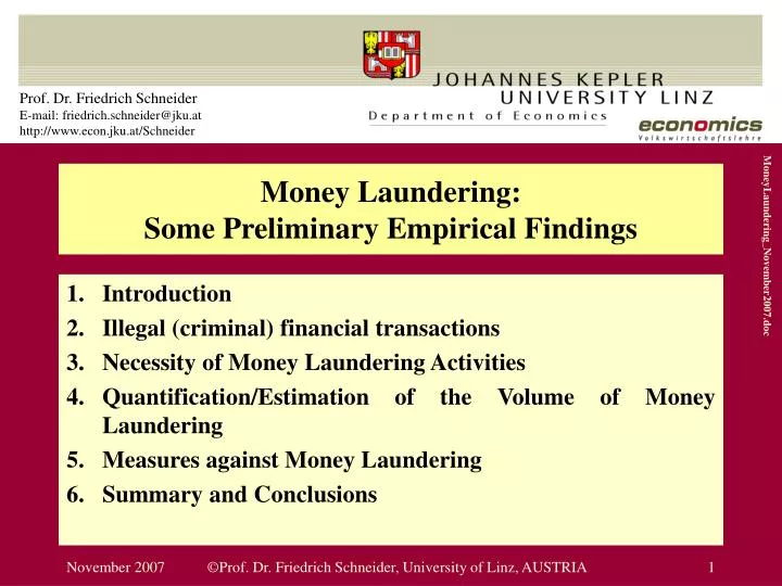
Prof. Dr. Friedrich Schneider E-mail: friedrich.schneider@jku.at http://www.econ.jku.at/Schneider. Money Laundering: Some Preliminary Empirical Findings. MoneyLaundering_November2007.doc. Introduction Illegal (criminal) financial transactions Necessity of Money Laundering Activities

E N D
Prof. Dr. Friedrich SchneiderE-mail: friedrich.schneider@jku.athttp://www.econ.jku.at/Schneider Money Laundering: Some Preliminary Empirical Findings MoneyLaundering_November2007.doc • Introduction • Illegal (criminal) financial transactions • Necessity of Money Laundering Activities • Quantification/Estimation of the Volume of Money Laundering • Measures against Money Laundering • Summary and Conclusions ©Prof. Dr. Friedrich Schneider, University of Linz, AUSTRIA
1. Introduction • The term „Money Laundering” originates from the US describing the Mafia’s attempt to “launder” illegal money via cash-intensive washing salons in the 30s, which where controlled by criminal organizations. • The IMF estimates, that 2-5% of the world gross domestic product (GDP) stems from illicit (criminal) sources. • The goal of this lecture is to undertake a first attempt, to shed some light about the size and development of money laundering and its techniques. ©Prof. Dr. Friedrich Schneider, University of Linz, AUSTRIA
2. Illegal (criminal) financial transactions • Apart from the “official” economy there exists an “Underground Economy”, which characterizes an illegal economy including all sorts of criminal activities, which are in conflict with the legal system, e.g. organized crime or drug dealing. • Opposite to these classical criminal activities, shadow economy activities mean the production of (in principle) legal goods and services with an value added for the official economy and where the illegality comes from avoiding taxes and social security payments and violating labour market regulations. • Shadow economy and underground (criminal) economy are quite different activities, which can not be summed up to one underground economy because the latter usually produces no positive value added for an economy. ©Prof. Dr. Friedrich Schneider, University of Linz, AUSTRIA
Table 2.2: Quantification of Money Laundering Volume – Part 1 Source: own calculations and reference list. ©Prof. Dr. Friedrich Schneider, University of Linz, AUSTRIA
Table 2.2: Quantification of Money Laundering Volume – Part 2 Source: own calculations and reference list. ©Prof. Dr. Friedrich Schneider, University of Linz, AUSTRIA
Figure 2.1: Organized Crime and their main areas in Central Europe Organized Crime – Main Fields Percentage in Central Europe ( Average 2000 - 2003) 40 10 15 5 10 20 Drugs Property Economy Violence Nightlife Weapons Drug - related Investment Armed Procuration Theft Nuclear Crime fraud Robbery Prostitution Illegal Car Economic Protection Illegal Break of Narcotics Movement Subsidy Fraud Money Gambling Embargo Burglary Payment Human Kidnapping Receiving Fraud Trafficing leads to Money Laundering Source: Siska, 1999, p. 13 and own calculations. ©Prof. Dr. Friedrich Schneider, University of Linz, AUSTRIA
Figure 2.2: Organized Crime – Main Fields (Central Europe, av. 2000-2003) Source: Siska, 1999, p. 13 and own calculations. ©Prof. Dr. Friedrich Schneider, University of Linz, AUSTRIA
3. Necessity of Money Laundering Activities • According to some estimations, the total turnover of organized crime actually reaches figures between 1,200 billion and 2,1 trillion USD in 2003 and the worldwide volume of money laundering “from drug business” obtains 810 billion in 2003. • Money laundering is necessary, because 2/3 of all illegal transactions are done by cash, as cash leaves no traces on information carriers like documents or bank sheets. ©Prof. Dr. Friedrich Schneider, University of Linz, AUSTRIA
4. Quantification/Estimation of the Volume of Money Laundering 4.1. General Remarks • Apart from a first major difficulty of diverging definitions of the term „money laundering“ on the national and the international level a second one arises, as particularly the transaction-intensive layering stage can lead exceedingly to potential double and multiple counting problems. • Furthermore many estimates (or guestimates) quite often are made for specific areas (e.g. drug profits) or are based on figures that are wrongly quoted or misinterpreted or just invented without a scientific base! ©Prof. Dr. Friedrich Schneider, University of Linz, AUSTRIA
4. Quantification/Estimation of the Volume of Money Laundering 4.1. General Remarks (cont.) • We make a distinction between direct and indirect methods: • Direct methods focus on recorded (“seized”/confiscated) illegal payments from the public authorities. However, to get an overall/total figure one has to estimate the much bigger (undetected/“Dunkelziffer”) volume. Methods, which are used are the discrepancy analysis of international balance of payment accounts, or of changes in cash stocks of national banks. • Indirect methods try to identify money laundering activities with the help of causes and indicators. First, the various causes (e.g. the various criminal activities) and indicators (confiscated money, prosecuted persons) are identified, and second an econometric estimation is undertaken. ©Prof. Dr. Friedrich Schneider, University of Linz, AUSTRIA
4. Quantification/Estimation of the Volume of Money Laundering 4.2. Econometric and DYMIMIC Procedures • In the DYMIMIC estimation procedure money laundering is treated as a latent (i.e. unobservable) variable. This estimation procedure uses various causes for money laundering (i.e. various criminal activities) and indicators (confiscated money, prosecuted, persons, etc.) to get an estimation of the latent variable. • One big difficulty of this method is, that one gets only relative estimated values of the size of money laundering and one has to use other estimations in order to transform/calibrate the relative values from the DYMIMIC estimation into absolute ones. ©Prof. Dr. Friedrich Schneider, University of Linz, AUSTRIA
4. Quantification/Estimation of the Volume of Money Laundering 4.2. Econometric and DYMIMIC Procedures – Cont. • A DYMIMIC estimation of the amount of money laundering or profits from criminal activities for 20 OECD countries over the years 1994/95, 1997/98, 2000/2001, 2002/2003 and 2003/2004 is done. • Theoretically we expect that the more illegal (criminal) activities (e.g. dealing with drugs, illegal weapon selling, increase in domestic crimes, etc.) occur, the more money laundering activities will take place, ceteris paribus. • The more inequal the income distribution and the lower official GDP per capita is, the higher money laundering activities will be, ceteris paribus. • The better the legal system is functioning the less money will be laundered, ceteris paribus. ©Prof. Dr. Friedrich Schneider, University of Linz, AUSTRIA
Figure 4.1: DYMIMIC estimation of the amount of money laundering for 20 highly developed OECD countries, 1994/95, 1997/98, 2000/2001 and 2002/2003 Functioning of the legal System Index: 1=worst, and 9=best -0.043*(2.10) Amount of confiscated money +0.380**(2.86) Criminal activities of illegal weapon selling +0.234**(3.41) Amount of Money Laundering or profits from criminal activities Lagged endogenous variable:+0.432*(2.20) Criminal activities of illegal drug selling +0.315**(3.26) Cash per capita +1.00 (Residuum) Criminal activities of illegal trade with human beings +0.217*(2.23) Prosecuted persons(number of persons) -0.264 (*)(-1.79) Criminal activities of faked products +0.102(1.51) Test-Statistics:RMSEA a) = 0.002 (p-value 0.884)Chi-squared b) = 16.41 (p-value 0.914)TMCV c) = 0.046AGFI d) = 0.710D.F. e) = 42a) Steigers Root Mean Square Error of Approximation (RMSEA) for the test of a close fit; RMSEA < 0.05; the RMSEA-value varies between 0.0 and 1.0.b) If the structural equation model is asymptotically correct, then the matrix S (sample covariance matrix) will be equal to Σ (θ) (model implied covariance matrix). This test has a statistical validity with a large sample (N ≥ 100) and multinomial distributions; both is given for this equation using a test of multi normal distributions.c) Test of Multivariate Normality for Continuous Variables (TMNCV); p-values of skewness and kurtosis.d) Test of Adjusted Goodness of Fit Index (AGFI), varying between 0 and 1; 1 = perfect fit.e) The degrees of freedom are determined by 0.5 (p + q) (p + q + 1) – t; with p = number of indicators; q = number of causes; t = the number for free parameters. Criminal activities of fraud, computer crime, etc. +0.113(1.62) Domestic crime activities +0.156*(2.43) Income distributionGini coefficient -0.213(*)(1.89) Per capita income in USD - 0.164(1.51) ©Prof. Dr. Friedrich Schneider, University of Linz, AUSTRIA
Table 4.1: DYMIMIC Calculations of the Volume of Money Laundering Source: Own calculations. ©Prof. Dr. Friedrich Schneider, University of Linz, AUSTRIA
Figure 4.2: DYMIMIC Calculations of the Volume of Money Laundering ©Prof. Dr. Friedrich Schneider, University of Linz, AUSTRIA
Table 4.3: Fight against money laundering in Austria and Germany Source: Own calculations (indirect analysis on basis of estimates on shadow economy and class. criminal activities); and Siska, Josef, 1999; BMI, 2003 and 2005; FIU 2005 und 2006. ©Prof. Dr. Friedrich Schneider, University of Linz, AUSTRIA
Figure 4.3: Fight against money laundering in Austria and Germany - Sum of criminal cash flow Germany Source: Own calculations (indirect analysis on basis of estimates on shadow economy and class. criminal activities); Siska, Josef, 1999; BMI, 2003 and 2005; FIU 2005 und 2006. ©Prof. Dr. Friedrich Schneider, University of Linz, AUSTRIA
Figure 4.4: Fight against money laundering in Austria and Germany - Sum of criminal cash flow Austria and Sum of “frozen money” Austria Source: Own calculations (indirect analysis on basis of estimates on shadow economy and class. criminal activities); Siska, Josef, 1999; BMI, 2003 and 2005; FIU 2005 und 2006. ©Prof. Dr. Friedrich Schneider, University of Linz, AUSTRIA
4. National estimations of the financial size of organized crime and money laundry Table 4.3: Shadow economy and underground economy in Germany from 1996 to 2006 ©Prof. Dr. Friedrich Schneider, University of Linz, AUSTRIA
4. National estimations of the financial size of organized crime and money laundry Table 4.4: Shadow economy and underground economy in Italy, France and Great Britain from 1996 to 2006 1) in % of official GDP ©Prof. Dr. Friedrich Schneider, University of Linz, AUSTRIA
4. Quantification/Estimation of the Volume of Money Laundering 4.3. The 10%-Rule of FATF The FATF (Financial Action Task Force) uses the following rule of thumb: • On basis of the estimated annual turnovers on retail trade level, the assumption is made that the confiscated amount is 10 per cent of all drugs floating around. • Knowing that the operating cost quota (relating to sales turnover) is roughly 60 per cent, profits/turnovers of drug trafficking can be estimated: In the year 1997 the FATF “estimated” a total world drug-turnover of approx. 300 billion USD, 120 billion USD profits thereof and 85 billion USD were classified to be relevant for money laundering. ©Prof. Dr. Friedrich Schneider, University of Linz, AUSTRIA
5. Measures against Money Laundering5.1. The Financial Action Task Force (FATF) • The Financial Action Task Force (FATF), an international organization, has the main task to fight against money laundering and terrorism financing, consisting of 33 member countries. The FATF tries to “hunt” the non-cooperative countries with the help of a “name and shame” policy by publishing a “black list”. • Moreover, the FATF is trying to combat money laundering internationally by means of typologies and 40 recommendations (international standards). Currently only Myanmar and Nigeria are still quoted on FATF’s black list. ©Prof. Dr. Friedrich Schneider, University of Linz, AUSTRIA
5. Measures against Money Laundering5.2. Austria • The main element of the existing money laundering precautions is formed by the so called “Know your Customer” principle; the FIU (Austrian Financial Intelligence Unit) has to be informed by all affected parties (banks, insurance companies, etc.) as soon as a suspect exceeds standardized limits in all financial business. • By banning anonymous savings bank books, identifying customers and obliging to store numerous documents etc. obligated parties comply with the “Know Your Customer” principle. ©Prof. Dr. Friedrich Schneider, University of Linz, AUSTRIA
5. Measures against Money Laundering5.3. Germany • In 2002 Germany established a Competence Centre named „Zentralstelle für verfahrensunabhängige Finanzer-mittlung“ to fight money laundering. • In addition, the control mechanism over financial transactions were extended combined with the establishment of a central database at the “Bundesauf-sichtsamt für Kreditwesen” in order to visualize cash flow of terrorism and money laundering organizations. • The authorization and the activity range of the current supervisory body (eg „Bundesaufsichtsamt für Wertpapier-handel“ oder „Bundesaufsichtsamt für Versicherungs-wesen“) was extended. ©Prof. Dr. Friedrich Schneider, University of Linz, AUSTRIA
6. Summary and Conclusions6.1. Summary • First, a differentiation is made between classical shadow economy and classical underground (crime) activities, arguing that on the one side shadow economy activities provide an extra value added of (in principal legal) goods and services, and on the other side typical crime activities produce no positive value added for the official economy. • Second, the necessity of money laundering is explained as since nearly all illegal (criminal) transactions are done by cash. Hence, this amount of cash must be laundered in order to have some “legal” profit. ©Prof. Dr. Friedrich Schneider, University of Linz, AUSTRIA
6. Summary and Conclusions6.1. Summary – Cont. • With the help of a DYMIMIC estimation procedure, the amount of money laundering are estimated using as causal variables e.g. various types of criminal activities, and as indicators, e.g. confiscated money. • The volume of laundered money or profits from criminal activities was for these 20 OECD countries in the year 1995 503 billions USD and increased in 2006 to 1,106 billions USD. • The worldwide money laundering turnover was in 2001 800 billion USD and increased in 2006 to 1,700 billion USD. ©Prof. Dr. Friedrich Schneider, University of Linz, AUSTRIA
6. Summary and Conclusions6.2. Conclusions Four preliminary conclusions: • Money laundering is extremely difficult to tackle. It’s defined almost differently in every country, the measures taken against it are different and vary from country to country. (2) To get a figure of the extent and development of money laundering over time is even more difficult. This paper tries to undertake some own estimations with the help of a latent estimation procedure (DYMIMIC) and shows that money laundering has increased from 1995 503 billion USD to 1,700 billion USD in 2006 for 20 OECD countries. ©Prof. Dr. Friedrich Schneider, University of Linz, AUSTRIA
6. Summary and Conclusions6.2. Conclusions – Cont. (3) To fight against money laundering is also extremely difficult, as we have no efficient and powerful international organizations, which can effectively fight against organized crime and money laundering. (4) Hence, this paper should be seen as a first start/attempt in order to shed some light on the grey area of money laundering and to provide some better empirical bases or taking more efficient measures against money laundering. ©Prof. Dr. Friedrich Schneider, University of Linz, AUSTRIA
Appendix 1: Multiple Indicators, Multiple Causes (MIMIC) approach The MIMIC approach explicitly considers several causes, as well as the multiple effects of the informal economy. The methodology makes use of the associations between the observeable causes and the observable effects of an unobserved variable, in this case the informal economy, to estimate the unobserved factor itself. Formally, the MIMIC model consists two parts: • The structural equation model describes the „relationship“ among the latent variable (informal economy = IE) and its causes. • The measurement model represents the link between the latent variable IE and its indicators; i.e. the latent varialble (IE) is expressed in terms of observable variables. ©Prof. Dr. Friedrich Schneider, University of Linz, AUSTRIA
Appendix 1: Multiple Indicators, Multiple Causes (MIMIC) approach The model for one latent variable (IE) can be described as follows: IE = γ‘ x + ν (1) Structural equation model γ =λ IE + ε (2) Measurement model where IE is the unobservable scalar latent variable (the size of the informal economy), γ‘ = (γ1…, γp) is a vector of indicators for IE, x‘ = (x1,…xq) is a vector of causes of IE, λ and γ are the (px1) and (qx1) vectors of the parameters and ε and ν are the (px1) and scalar errors. ©Prof. Dr. Friedrich Schneider, University of Linz, AUSTRIA
Appendix 1: Figure 1: General structure of a MIMIC model Causes Indicators λ1 γ1 x1t y1t – ε1t γ2 λ2 x2t y2t – ε2t IEt γq … … λp xqt ypt – εpt ©Prof. Dr. Friedrich Schneider, University of Linz, AUSTRIA
Appendix 1: Multiple Indicators, Multiple Causes (MIMIC) approach Equation (1) links the informal economy with ist indicators or symptoms, while equation (2) associates the informal economy with ist causes. Assuming that these errors are normally distributed and mutually uncorrelated with var(ν) = σ2 ν and cov(ε) = Θε, the model can be solved for the reduced form as a function of observable variables by combining equations (1) and (2): γ = π x + μ (3) where π = λγ‘ , μ = λν + ε and cov(μ) = λλ‘ σ2ν + Θε. ©Prof. Dr. Friedrich Schneider, University of Linz, AUSTRIA
Appendix 1: Multiple Indicators, Multiple Causes (MIMIC) approach Because γ and x are observable data vectors, equation (3) can be estimated by maximum likelihood estimation using the restrictions implied in both the coefficient matrix π and the covariance matrix of the error μ. Since the reduced form parameters of equation (3) remain unaltered when λ is multiplied by a scalar and γ and σ2 ν are divided by the same scalar, the estimation of (1) and (2) requires a normalization of the parameters in (1), and a convenient way to achieve this is to constrain one element of λ to some pre-assigned value (quite often 1). Since the estimation of λ and γ is obtained by constraining one element of λ to some arbitrary value, it is useful to standardize the regression coefficients ^λ and ^γ as follows: ^λs = ^λ (^σIE / ^σγ) ^γs = ^γ (^σx /^σIE ) ©Prof. Dr. Friedrich Schneider, University of Linz, AUSTRIA
Appendix 1: Multiple Indicators, Multiple Causes (MIMIC) approach The standardized coefficient measures the expected change in the standard-deviation units of the dependent variable due to a one standard-deviation change fo the given explanatory variable when the other variables are held constant. Using the estimates of the γs vector and setting the error term ν to its mean value of zero, the predicted ordinal values for the informal economy (IE) can be estimated by using equation (2). Then, by using information regarding the specific value of informal activity for some country (if it is a cross country study) or for some point in time (if it is a time series study), obtained from some other source, the within-sample predictions for IE can be converted into absolute series. ©Prof. Dr. Friedrich Schneider, University of Linz, AUSTRIA