Download
1 / 56
570 likes | 745 Views
Chapter 5 Inventory in the Logistics System. Overview and Importance Functional Types Reasons to Carry Inv. Inv. Cost Types Classifying Inv. Evaluating Effectiveness Trends in Inv. Mgt. Potential Inventory Positions. R. DC. R. S. 1. 1. DC. R. S. 2. 2. Plant W/H. Plant/Mfg.

E N D
Chapter 5Inventory in the Logistics System • Overview and Importance • Functional Types • Reasons to Carry Inv. • Inv. Cost Types • Classifying Inv. • Evaluating Effectiveness • Trends in Inv. Mgt.
Potential Inventory Positions R DC R S 1 1 DC R S 2 2 Plant W/H Plant/Mfg W/H DC R S 3 3 S DC R n n R
Overview and Importance • Inventory - “Double-Edge Sword” • Inventory as a Percent of U.S. GNP (next slide) • Factors Affecting Aggregate Expenditures on Inventory • Transportation deregulation • Communications and information technologies • Improvements in “inventory velocity” • Product proliferation • Interest rates/cost of capital
Key Inventory Trends • Dollar Value of U.S. Inventory Continues to Rise • Inventory/GNP or Inventory/Sales Ratios are Decreasing • Inventory Carrying Costs are Increasing as Percent of Total Distribution Cost • Acquisition of Higher-Value, Lower-Weight Products Will Result in Higher Costs of Carrying Inventory • Reinforced Need for Effective Approaches to Inventory Segmentation, such as ABC Analysis
Example: Inventory Calculations • Inventory Carrying Cost = Dollar value of inventory x percentage carrying cost • Example If dollar value of inv. = $50,00 And carrying cost = 22% of product value Then Inventory Carrying Cost = =
Sales Average Inventory $38.8 billion $8.8 billion Example: Inventory Calculations (Continued) • Inventory Turnover = • Example: K-Mart 1992 Sales = $38.8 billion 1992 Avg. Inv. = $8.8 billion Inventory Turnover = = turns/year
Avg. Inv. Sales Example: Inventory Calculations (Continued) = x 365 • Average Day’s Inventory on Hand • Example: K-Mart (cont.) 1992 Sales = $38.8 billion 1992 Avg. Inv. = $8.8 billion Avg. Day’s IOH = $8.8 x 365 $38.8 = Days
Saving Inventory Dollarsby Increasing Inventory Turns Inventory Carrying Cost Inventory Turns
Functional Types of Inventory • Cycle stock • In-process stock (Goods-In-Process, WIP, In-Transit) • Safety (buffer) stock • Demand and/or lead time uncertainty • Customer service • Seasonal stock • Promotional stock • Sales and deals • Speculative stock • Fluctuating price and/or availability • When using long supply lines • Dead stock
Inventory Costs Carrying Costs Expected Stockout Costs Order/ Setup Costs
Inventory Carrying Costs • Capital Costs • Expressed as percentage of product value • Based on value of average inventory • rate is most appropriate • =minimum rate of return on new investments • Observations • Interest rates not entirely valid • Industry averages misleading • Most companies calculate incorrectly • Rule of thumb of 25% can be very misleading • Range of percentages found in textbooks can justify nearly any inventory policy
Inventory Carrying Costs (Continued) • Storage Space Cost • Consider only variable portion • Will differ between public and private warehousing • Inventory Service Cost • Inventory Risk Cost • Deterioration • Obsolescence • Damage • Pilferage and theft
#1 #2 #3 #4 $5 $10 $15 $20 Calculating Carrying Cost • Identify Item Value • FIFO (higher inventory valuation when prices are rising - and vice-versa) • LIFO (lower inventory valuation when prices are rising - and vice-versa) • Average Cost
Measure Carrying Cost Components Example: Capital Cost 20% Storage Space 8% Inv. Service 4% Inv. Risk 6% 38% Multiply Percent by Value Example: Value = $50 per item Inventory Carrying Cost = ($50)(.38) = $19.00 per item/per year Calculating Carrying Cost (Continued)
Rationale for Carrying Inventory • Purchase Economies • Transportation Savings • Reduce Risk
Order / Setup Cost Annual Cost ($) Size of Order (units) • Note: Order / setup cost reflects: • Fixed costs (e.g., information and communications technology) • Variable costs (e.g., reviewing stock levels, order processing/ • preparation expense, etc.)
Measuring Effectiveness of Inventory Management • End-Users Satisfied? • Frequent Need for “Backordering” or “Expediting? • Order Cancellations? • Inventories Available at “Right” Locations? • Measures of Inventory Turnover • Too low? • Too high?
Symptoms of Poor Inventory Mgt • Increasing back-order status • increasing dollar investments in inventory with back-orders remaining constant • High customer turnover rate • Increasing number of orders being canceled • Periodic lack of sufficient storage space • Wide variance in inventory turnover among distribution centers and among major inventory items • deteriorating relationships with middlemen as typified by dealer cancellations and declining orders • Inventories rising faster than sales • Customers not satisfied • Inventory turnover too low
Current Inventory Trends • Shifting Inventory Positioning • From retailers to distributors • From distributors to manufacturers and suppliers • Out of the system whenever possible • Accelerating use of point-of-sale (POS) and real-time information to make inventory replenishment decisions; company processes for order processing and inventory management are being integrated • New providers of inventory services • Wholesalers in support of retailers • 3rd party/contract logistics suppliers • Other supplier firms in complementary businesses • Search for effective, contemporary approaches to inventory management and control
Chapter 6Inventory Decision Making • Fundamental Approaches • Fixed Order Quantity • Fixed Order Interval • Inventory at Multiple Locations • Time Based Approaches • QR and ECR • Comparison of Various Methods
Fundamental Approaches • Nature of Demand • Independent vs. Dependent • Driver or Trigger of Order • Pull vs. Push or Hybrid • Company or Supply Chain Philosophy • Systemwide vs. Single-Facility Solution
Fixed Order Quantity (EOQ) Approach • Key Questions: • How much to reorder? • When to reorder? • Total cost? • Two Tradeoffs • Principle Assumptions (CBL, pp. 195) • Demand is continuous, constant, and known in advance • Lead time is constant and known in advance • Price of item is independent of order quantity
Basic Tradeoffs • As order quantity (EOQ) increases: • Annual inventory carrying cost also increases • Annual ordering cost decreases • Example: CBL, pp. 196-198 Cost Annual Cost Cost Size of Order Quantity
600 400 200 Sawtooth Models Units 1/2Q 20 40 60 Time
Mathematical Formulation • Total Annual Cost = Annual Inventory Carrying Cost + Annual Ordering Cost • Letting TAC = Annual Total Cost ($) R = Annual demand (units) A = Cost of placing a single order ($) V = Value of one unit of inventory ($) W = Inventory carrying cost as a % of product value Q = EOQ • Then: TAC = 1/2 QVW + A (R/Q) • and: the EOQ that minimizes the TAC is:
Example of EOQ R = Annual demand = 600 units A = Order cost = $4/order V = Product value = $240/unit W = inventory carrying cost = 20% = 0.20 10 units =
Example of TAC: R = Annual demand = 600 units A = Order cost = $4/order V = Product value = $240/unit W = inventory carrying cost = 20% = 0.20 Then: TAC = 1/2 QVW + A (R/Q) 1/2 (10) (240) (0.20) + (4) (600/10) 240 + 240 $480
Determining the Reorder Point The Goal is to have a shipment of EOQ units to arrive as the Balance-On-Hand = 0 Reorder Point (ROP) = minimum amount of inventory to last during the replenishment or lead time = [Lead time length (in days)] X [Demand per day (in units per day)] Continuing Example: (Assume 300 days per year) Lead time length = 12 days Then Demand per day = 600 / 300 = 2 units/day ROP = ( 12 days) ( 2 units/day) ROP = 24 units Additional exercises to do at home: CBL, pp. 230, #7 and 8
EOQ Review • Perhaps the most well-know, traditional approach to managing inventory • computes an “optimum’ value for the economic order quantity (EOQ) based on a trade-off of two types of cost: • Inventory carrying cost • Ordering cost or setup cost • Replenishment orders placed when inventory-on-hand reaches a pre-determined “ROP” • currently declining in popularity and frequency of use: • Too much emphasis on carrying inventory • Not very useful for systems with multiple distribution centers • Greater emphasis today on approaches which “synchronize” delivery of shipments with timing of actual need (e.g., JIT)
Related Concepts • “Two-bin” system • “Min-max” system • demand may occur in larger increments than with the traditional EOQ approach
EOQ in Condition of Uncertainty • Uncertainty = variation in demand and/or lead time • Requires holding of safety stock inventory • Policy: Cost of carrying safety stock should be balanced with expected cost of stockouts • Average inventory = 1/2 EOQ + Safety Stock • skip CBL, pp. 205-211 on “how to calculate example”
Inventory Model UnderConditions of Uncertainty • EOQ is still the amount ordered each time • Assumes that over time, uncertainty periods balance out Inventory Level (Units) Qm ROP Safety Stock Time
Fixed Order Interval • Involves ordering of inventory at fixed or regular intervals • Amount order depends on how much is on-hand at the time of ordering (NOT EOQ) • Implications: • Does not require close surveillance of inventory levels • Inventory monitoring less expensive • Over time, it results in higher safety stock levels
$4,000 $3,000 Units $2,000 $1,000 1 2 3 4 5 1 2 3 4 5 1 2 3 4 5 1 2 Time (weeks) Fixed Interval Modal
Inventory at Multiple LocationsSquare Root Rule • How does total inventory change as the number of stocking points changes? • Let: n1 = number of existing facilities n2 = number of future facilities x1 = total inventory in present facilities x2 = total inventory in future facilities
= 50,000 = 50,000 Example: Square Root Law • Currently, the company has 50,000 units located in 3 facilities. The company plans to expand to 27 locations. How will this affect total inventory? 150,000 units =
Time Based Approaches to Replenishment Logistics • Continuous Replenishment (CRP) Inventory Systems • Flow-Through Logistics Systems • Pipeline (Supply Chain) Logistics Organizations • Pipeline Performance Measures Note: See Figure 6-12, CBL page 216 for further detail.
Quick Response (QR) • QR is a method of maximizing the efficiency of the supply chain by reducing inventory investment where partners commit to meet specific service performance criteria. • shorter, compressed time horizons • Real-time information by SKU • Seamless logistics network • Partnership relationships throughout the supply chain • Commitment to Quality
QR Profit Sources Faster Order Placement Shorter Lead Times Rapid Reaction to Demand More Reliable Lead Times Fast Response to Sales Trends Higher Sales Lower Markdowns Reduced Cycle Stock Reduced Safety Stock Lower Markdowns Higher Sales Greater Profitability Reduced Total Channel Costs
QR Overall Cost/Revenue Implications $ Total Cost Traditional QR
Manufacturing Transportation Materials Handling Inventory QR Overall Cost/Revenue Implications Revenue $ Total Cost Traditional QR
Time Savings from QR 66 46 21
Efficient Consumer Response (ECR) Timely, accurate, paperless information flow Consumer Household Supplier Distributor Retail Store Smooth, continual product flow matched to consumption Source: Kurt Salmon Associates, Inc. Efficient Consumer Response: Enhancing Consumer Value in the Grocery Industry
ECR • Components • Category management (Managing product groups as strategic business units) • Integrated electronic data interchange (EDI) • Activity-Based Costing (ABC) • Continuous replenishment programs • Flow-through cross-dock replenishment • Benefits • Better - products, assortments, in-stock performance, and prices • Leaner, faster, more responsive, less costly supply chain • Improved asset utilization