Deconvolution: The Power of CLEAN Algorithm
Learn the ins and outs of deconvolution in astronomy, from the works of CLEAN algorithm to MEM deconvolution. Discover how these techniques help reveal hidden sources in the sky plane using parallel cleaning and overcoming challenges. Explore the efficacy, limitations, and solutions of CLEAN algorithm, parallel cleaning, and MEM method.

Deconvolution: The Power of CLEAN Algorithm
E N D
Presentation Transcript
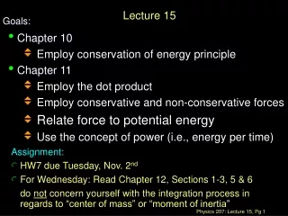
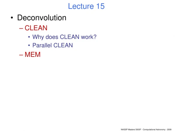
Lecture 15 • Deconvolution • CLEAN • Why does CLEAN work? • Parallel CLEAN • MEM
Deconvolution. • How can we go from • this • to this? • Deconvolution in the sky plane implies interpolation or reconstruction of missing values in the UV plane. • But we, the human observer, can look at the top image and just ‘know’ that it is 2 point sources on a blank field.
CLEAN • The following ‘naive’ algorithm gives surprisingly good results: • Find the brightest pixel xb,yb in the dirty image. • Measure its brightness I(xb,yb). • Subtract λI(xb,yb)B(x-xb,y-yb) from the image, where λ is a number in the approximate range 0.01 to 0.2. • Repeat until satisfied. • This is known as the CLEAN algorithm. The successive numbers λI are called clean components.
Problems with CLEAN: • Mathematicians don’t like CLEAN. They say it ought not to work. There are lots of papers out there proving it doesn’t. • But it does work, good enough for rough-and-ready astronomers, anyway. • This is because the real sky obeys strong constraints: • Nearly always there are just a few smallish bright patches on a blank background; • Negative flux values don’t occur in the real sky. • CLEAN doesn’t work really well on extended sources – can get ‘clean stripes’ or ‘bowl’ artifacts. • It is difficult to know when to stop CLEANing. Too soon, and you are missing flux. Too late, and you are just cleaning the noise in your image.
More problems with CLEAN: • Sources which vary in flux over the duration of the observation. • Solution: cut the observation into shorter chunks, clean separately, then recombine. • Clunky, loses sensitivity. • ‘Parallel’ cleaning works well though. • (Only relevant for wide-band case:) different sources have different shapes of spectrum. • Parallel cleaning is also good for this – even when sources vary both in frequency and time! • Sources which aren’t located at the centre of a pixel. Fixes: • Re-centre on each source, then CLEAN them away. • You guessed it – parallel cleaning can also help.
Parallel CLEAN: • First developed to cope with wide-band imaging. The fundamental paper is: • The basic idea is to construct a number of dirty beams, the jth beam (starting at j=0) by setting Vj(ν) to (ν/ν0)j/j! then FTing. Eg V0=1, V1=ν/ν0, V2=(ν/ν0)2/2, etc. Since the Vjs form a Taylor series, any spectrum can be approximated by a sum of Vjs; thus any source by a sum of Bjs. Sault R J & Wieringa M H: A&A Suppl. Ser. 108, 585 (1994)
Description of the problem: an example. S ν If both point sources have identical spectra, there is no problem. S ν
Description of the problem: an example. More realistic: different spectra: S ν S ν This will not clean away.
The Sault-Wieringa algorithm: νref νref νref νref ν ν ν ν 0th order S + Taylor expansion 1st order + A source spectrum: 2nd order etc…
Taylor-term beams max = 1.0 max = 0.02 max = 0.01 max = 0.004 0th order 1st order 2nd order 3rd order
A simulation to test this: 19 point sources from 0.001 to 1 Jy Spectra: cubics, with random coefficients. eg ν (GHz)
Alternate cleaning:(i) 1000 cycles of standard clean …not good.
Alternate cleaning:(ii) each spectral channel cleaned, then co-added. …pretty good, but do we lose faint sources?
S-W clean to various orders (All 1000 cycles with gain (λ) = 0.1) 0th order (equivalent to standard clean)
S-W clean to various orders 1st order
S-W clean to various orders 2nd order
S-W clean to various orders 3rd order Not much left but numerical noise.
Time-varying sources: Source constant in time Source flux varying with time
Time-varying sources: I M Stewart et al – paper in preparation!
MEM – the Maximum Entropy Method. • (Content for this slide pretty much copied from T. Cornwell, chapter 7, NRAO 1985 Synthesis Imaging Summer School. I haven’t studied ME myself.) • What does entropy mean in this context? • “Something which, when maximized, produces a positive image with a compressed range of pixel values.” • An example: maximize • I guess we would need to read Narayan and Nityananda 1984 to figure out what e is. I is the image we end up with M is our ‘best guess’ starting image.