Download
1 / 145
1.48k likes | 1.72k Views
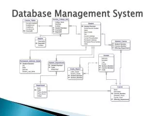
Database Management System Recent Advances. By Prof. Dr.O.P . Vyas M.Tech .(CS), Ph.D. ( I.I.T. Kharagpur ) DAAD Fellow ( Germany ) AOTS Fellow ( Japan) Professor & Head ( Computer Science) Pt. R.S. University Raipur (CG)

E N D
Database Management SystemRecent Advances By Prof. Dr.O.P. Vyas M.Tech.(CS), Ph.D. ( I.I.T. Kharagpur ) DAAD Fellow ( Germany ) AOTS Fellow ( Japan) Professor & Head ( Computer Science) Pt. R.S. University Raipur (CG) [ Visiting Prof. – Rostock University Germany ]
Contents ADBMS • Concepts of Association Rule Mining • ARM Basics • Problems with Apriori • Apriori Vs. FP tree • ARM Variants • Classification Rule Mining • Classification techniques • Classifiers • Various classifiers • Classification & Prediction • Classification accuracy • Mining Complex data types • Complex data types • Data mining Process & Integration with existing Technology
Data Mining Association Mining Clustering Analysis Classification Classification Techniques A:R:M: Techniques Asso.Classifiers Application domain Data Mining Functionalities
Retail shops are often interested in associations between different items that people buy. Someone who buys bread is quite likely also to buy milk A person who bought the book Database System Concepts is quite likely also to buy the book Operating System Concepts. Association information can be used in several ways. E.g. when a customer buysa particular book, an online shop may suggest associated books. Association rules: bread milk DB-Concepts, OS-Concepts Networks Left hand side: antecedent, right hand side: consequent An association rule is a pattern that states when Antecedent occurs, Consequent occurs with certain probability. Association Rules
Rules have an associated support, as well as an associated confidence. Support is a measure of what fraction of the population satisfies both the antecedent and the consequent of the rule. E.g. suppose only 0.001 percent of all purchases include milk and screwdrivers. The support for the rule is milk screwdrivers is low. We usually want rules with a reasonably high support Rules with low support are usually not very useful Confidenceis a measure of how often the consequent is true when the antecedent is true. E.g. the rule bread milk has a confidence of 80 percent if 80 percent of the purchases that include bread also include milk. Usually want rules with reasonably large confidence. A rule with a low confidence is not meaningful. Note that the confidence of bread milk may be very different from the confidence of milk bread, although both have the same supports. Association Rules (Cont.)
A.R.M model: data • A.R.M. was initially applied to Market Basket Analysis on transaction data of Supermarket sales. • I = {i1, i2, …, im}: a set of items. • Transactiont : • t a set of items, and tI. • Transaction Database T: a set of transactions T = {t1, t2, …, tn}.
Transaction data: supermarket data • Market basket transactions: t1: {bread, cheese, milk} t2: {apple, eggs, salt, yogurt} … … tn: {biscuit, eggs, milk} • Concepts: • An item: an item/article in a basket • I:the set of all items sold in the store • A transaction: items purchased in a basket; it may have TID (transaction ID) • A transactionaldataset: A set of transactions
Transaction data: a set of documents • A text document data set. Each document is treated as a “bag” of keywords doc1: Student, Teach, School doc2: Student, School doc3: Teach, School, City, Game doc4: Baseball, Basketball doc5: Basketball, Player, Spectator doc6: Baseball, Coach, Game, Team doc7: Basketball, Team, City, Game
The model: rules • A transaction t contains X, a set of items (itemset) in I, if Xt. • An association rule is an implication of the form: X Y, where X, Y I, and X Y = • An itemsetis a set of items. • E.g., X = {milk, bread, cereal} is an itemset. • A k-itemset is an itemset with k items. • E.g., {milk, bread, cereal} is a 3-itemset
Rule strength measures • Support: The rule holds with supportsup in T (the transaction data set) if sup% of transactionscontain X Y. • sup = Pr(X Y). • Confidence: The rule holds in T with confidence conf if conf% of tranactions that contain X also contain Y. • conf = Pr(Y | X) • An association rule is a pattern that states when X occurs, Y occurs with certain probability.
Mining Association Rules—An Example Let us take the Min. support 50% Min. confidence 50% For rule AC : support = support({AC}) = 50% confidence = support({AC})/support({A}) = 66.6% • A C(50%, 66.6%) • C A(50%, 100%) • The Apriori principle: Any subset of a frequent itemset must be frequent
The Apriori Algorithm • Join Step:Ckis generated by joining Lk-1with itself • Prune Step:Any (k-1)-itemset that is not frequent cannot be a subset of a frequent k-itemset • Pseudo-code: Ck: Candidate itemset of size k Lk : frequent itemset of size k L1 = {frequent items}; for(k = 1; Lk !=; k++) do begin Ck+1 = candidates generated from Lk; for each transaction t in database do increment the count of all candidates in Ck+1 that are contained in t Lk+1 = candidates in Ck+1 with min_support end returnkLk;
The Apriori Algorithm — Example Database D L1 C1 Scan D C2 C2 L2 Scan D L3 C3 Scan D
Generating rules from frequent itemsets • Frequent itemsets association rules • One more step is needed to generate association rules • For each frequent itemset X, For each proper nonempty subset A of X, • Let B = X - A • A B is an association rule if • Confidence(A B) ≥ minconf, support(A B) = support(AB) = support(X) confidence(A B) = support(A B) / support(A)
Generating association rules.. • Once the frequent itemsets from transactions in a database D have been found, it is straightforward to generate strong association rules from them ( where strong association rules satisfy both minimum support and minimum confidence). • To recap, in order to obtain A B, we need to have support(A B) and support(A) • All the required information for confidence computation has already been recorded in itemset generation. No need to see the data T any more. • This step is not as time-consuming as frequent itemsets generation.
Goal and key features • Goal: Find all rules that satisfy the user-specified minimum support (minsup) and minimum confidence(minconf). • Key Features • Completeness: find all rules. • No target item(s) on the right-hand-side • Mining with data on hard disk(not in memory)
Mining Association Rules in Large Databases • Association rule mining:Association rule can be classified into categories based on different criteria such as; 1. Based on types of Values handledin the rule, associations can be classified into Boolean Vs. quantitative. A Boolean association shows relationships between discrete (categorical) objects. A quantitative association is a multidimensional association. Example of quantitative association rule, where X is is a variable representing a customer Age (x,”30….39”) ^ income (X,”42k…48k) buys ( X, high resolution TV) Note that quantitative attributes, age and income have been discretized 2. Based on dimensions of data involved in the rule. Ex. Purchase (X, ‘computer’ ) Purchase (X, ‘financial software’) is a single dimensional association rule, and if date/time of purchase is added, it becomes multidimensional. 3. Multilevel Association Rule Mining 4. Multi Dimensional A.R.M.
uniform support reduced support Level 1 min_sup = 5% Milk [support = 10%] Level 1 min_sup = 5% Level 2 min_sup = 5% 2% Milk [support = 6%] Skim Milk [support = 4%] Level 2 min_sup = 3% Mining Multiple-Level Association Rules • Items often form hierarchies • Flexible support settings • Items at the lower level are expected to have lower support • Exploration of sharedmulti-level mining (Agrawal & Srikant@VLB’95, Han & Fu@VLDB’95)
Multi-level Association: Redundancy Filtering • Some rules may be redundant due to “ancestor” relationships between items. • Example • milk wheat bread [support = 8%, confidence = 70%] • 2% milk wheat bread [support = 2%, confidence = 72%] • We say the first rule is an ancestor of the second rule. • A rule is redundant if its support is close to the “expected” value, based on the rule’s ancestor.
Mining Multi-Dimensional Association • Single-dimensional rules: buys(X, “milk”) buys(X, “bread”) • Multi-dimensional rules: 2 dimensions or predicates • Inter-dimension assoc. rules (no repeated predicates) age(X,”19-25”) occupation(X,“student”) buys(X, “coke”) • hybrid-dimension assoc. rules (repeated predicates) age(X,”19-25”) buys(X, “popcorn”) buys(X, “coke”) • Categorical Attributes: finite number of possible values, no ordering among values—data cube approach • Quantitative Attributes: numeric, implicit ordering among values—discretization, clustering, and gradient approaches
Mining Association Rules in Large Databases • Mining single-dimensional Boolean association rules from transactional databases • The Apriori Algorithm- an influential algorithm for mining frequent itemsets for boolean association rules, it uses prior knowledge of frequent itemset properties. • Apriori employs an iterative approach known as a level-wise search, where k-itemsets are used to explore (k+1) itemsets. • First the set of frequent 1-itemsets is found. This set is denoted as L1. L1 is used to find the set of frequent 2-itemset, L2. And so on until no more frequent k-itemsets can be found. • The finding of each Lk requires one full scan of the database.
Many ARM algorithms • There are a large number of them!! • They use different strategies and data structures. • Their resulting sets of rules are all the same. • Given a transaction data set T, and a minimum support and a minimum confident, the set of association rules existing in T is uniquely determined. • Any algorithm should find the same set of rules although their computational efficiencies and memory requirements may be different. We study only one: the Apriori Algorithm
On Apriori Algorithm Seems to be very expensive • Level-wise search • K = the size of the largest itemset • It makes at most K passes over data • In practice, K is bounded (10). • The algorithm is very fast. Under some conditions, all rules can be found in linear time. • Scale up to large data sets • Clearly the space of all association rules is exponential, O(2m), where m is the number of items in I. • The mining exploits sparseness of data, and high minimum support and high minimum confidence values. • Still, it always produces a huge number of rules, thousands, tens of thousands, millions, ...
UCI KDD Archive http://kdd.ics.uci.edu • This is an online repository of large data sets which encompasses a wide variety of data types, analysis tasks, and application areas. • The primary role of this repository is to enable researchers in knowledge discovery and data mining to scale existing and future data analysis algorithms to very large and complex data sets. • . The archive is intended to serve as a permanent repository of publicly-accessible data sets for research in KDD and data mining. It complements the original UCI Machine Learning Archive , which typically focuses on smaller classification-oriented data sets.
ARM Implementations • Many implementations of Apriori Algorithm are available • http://www.cs.bme.hu/~bodon/en/apriori/ (APRIORI implementation of Ferenc Bodon) • http://www.csc.liv.ac.uk/~frans/KDD/Software/Apriori-T_GUI/aprioriT_GUI.html [ Apriori-T (Apriori Total) is an Association Rule Mining (ARM) algorithm, developed by the LUCS-KDD research team The code obtainable from this page is a GUI version that inludes (for comparison purpopses) implementations of Brin's DIC algorithm (Brin et al. 1997) and Toivonon's negative boarder ARM approach (Toivonen 1996) ] • http://www.csc.liv.ac.uk/~frans/KDD/Software/FPgrowth/fpGrowth.html ( Implementation of FP growth method ) • DBMiner is data mining system which runs on top of Microsoft SQL server 7.0 Plato system.
A.R.M. Implementations:Example • In DBMiner, three kinds of associations could be possibly mined: • Inter-dimensional association. Associations among or across two or more dimensions. Customer-Country("Canada") => Product-SubCategory("Coffee") i.e. Canadian customers are likely to buy coffee. 2. Intra-dimensional association. Associations present within one dimension grouped by another one or several dimensions. For example, if you want to find out which products customers in Canada are likely to purchase together: Within Customer-Country("Canada"): Product-ProductName("CarryBags") => Product-ProductName("Tents")i.e. Customers in Canada, who buy carry-bags, are also likely to buy tents. 3. Hybrid association. Associations combining elements of both inter- and intra-dimensional association mining. For example, Within Customer-Country("Canada"): Product("Carry Bags") => Product("Tents"), Time("Q3")i.e. Customers in Canada, who buy carry-bags, also tend to buy tents and do so most often in the 3rd quarter of the year (Jul, Aug, Sep).
Problems with the association mining • Single minsup: It assumes that all items in the data are of the same nature and/or have similar frequencies. • Not true: In many applications, some items appear very frequently in the data, while others rarely appear. E.g., in a supermarket, people buy food processor and cooking pan much less frequently than they buy bread and milk.
Rare Item Problem • If the frequencies of items vary a great deal, we will encounter two problems • If minsup is set too high, those rules that involve rare items will not be found. • To find rules that involve both frequent and rare items, minsup has to be set very low. This may cause combinatorial explosion because those frequent items will be associated with one another in all possible ways.
Is Apriori Fast Enough? — Performance Bottlenecks • The core of the Apriori algorithm: • Use frequent (k – 1)-itemsets to generate candidate frequent k-itemsets • Use database scan and pattern matching to collect counts for the candidate itemsets • The bottleneck of Apriori: candidate generation • Huge candidate sets: • 104 frequent 1-itemset will generate 107 candidate 2-itemsets • To discover a frequent pattern of size 100, e.g., {a1, a2, …, a100}, one needs to generate 2100 1030 candidates. • Multiple scans of database: • Needs (n +1 ) scans, n is the length of the longest pattern
Mining Frequent Patterns Without Candidate Generation FP-Tree(Frequent Pattern Tree) Algorithm. To break the two bottlenecks of Apriori series algorithms, some works of association rule mining using tree struc-ture have been designed. FP-Tree [Han et al. 2000], frequent pattern mining, is another milestone in the development of association rule mining, which breaks thetwo bottlenecks of the Apriori. The frequent itemsets are generated with only two passes over the database and without any candidate generation process. FP-Tree was introduced by Han et al in [Han et al. 2000]. By avoiding the candidate generation process and less passes over the database, FP-Tree is an order of magnitude faster than the Apriori algorithm. The frequent patterns generation process includes two sub processes: constructing the FT-Tree, and generating frequent patterns from the FP tree.
FP Tree • Compress a large database into a compact, Frequent-Pattern tree (FP-tree) structure • highly condensed, but complete for frequent pattern mining • avoid costly database scans • Develop an efficient, FP-tree-based frequent pattern mining method • A divide-and-conquer methodology: decompose mining tasks into smaller ones • Avoid candidate generation: sub-database test only! • Some Researchers have identified that when dataset is vary sparse then FP Tree has shown bottlenecks and Apriori has comparatively given better performance !!
{} Header Table Item frequency head f 4 c 4 a 3 b 3 m 3 p 3 f:4 c:1 c:3 b:1 b:1 a:3 p:1 m:2 b:1 p:2 m:1 Construct FP-tree from a Transaction DB TID Items bought (ordered) frequent items 100 {f, a, c, d, g, i, m, p}{f, c, a, m, p} 200 {a, b, c, f, l, m, o}{f, c, a, b, m} 300 {b, f, h, j, o}{f, b} 400 {b, c, k, s, p}{c, b, p} 500{a, f, c, e, l, p, m, n}{f, c, a, m, p} min_support = 0.5 • Steps: • Scan DB once, find frequent 1-itemset (single item pattern) • Order frequent items in frequency descending order • Scan DB again, construct FP-tree
Benefits of the FP-tree Structure • Completeness: • never breaks a long pattern of any transaction • preserves complete information for frequent pattern mining • Compactness • reduce irrelevant information—infrequent items are gone • frequency descending ordering: more frequent items are more likely to be shared • never be larger than the original database (if not count node-links and counts) • Example: For Connect-4 DB, compression ratio could be over 100
Mining Frequent Patterns Using FP-tree • General idea (divide-and-conquer) • Recursively grow frequent pattern path using the FP-tree • Method • For each item, construct its conditional pattern-base, and then its conditional FP-tree • Repeat the process on each newly created conditional FP-tree • Until the resulting FP-tree is empty, or it containsonly one path(single path will generate all the combinations of its sub-paths, each of which is a frequent pattern)
Market Basket Analysis: Purpose • The Supermarket revolution when first sparked off in the 1920s, one could not even dream of retailing as it exists today. By the1950s it had won acclaim and acceptance almost globally. This is one retailing sector that is spreading very fast in India. But still majority of retailing sector including this one is not properly managed. • Retailing management has been in focus for marketing strategists since long as organized retailing is assuming significant attention. M.B.A is one such effort. • In a supermarket retailing MBA has endeavored to study and analyze the combination of various items accumulated in a ‘Shopping Basket’ and was intended to establish Associationship between the various items bought by the customer. • Market basket analysis is a generic term for methodologies that study the composition of a basket of products (i.e. a shopping basket) purchased by a household during a single shopping trip. • The idea is that market baskets reflect interdependencies between products or purchases made in different product categories, and that these interdependencies can be useful to support retail marketing decisions.
MBA • Our data mining approach to super market business data will record all the supermarket transactions in a tabular form and appropriate algorithm will process the transaction data to provide significant Associationships of various items. • From a marketing perspective, the research is motivated by the fact that some recent trends in retailing pose important challenges to retailers in order to stay competitive. In fact, on the level of the retailer, a number of trends can be identified, including concentration, internationalization, decreasing profit margins and an increase in discounting. • Recently, a number of advances in data mining (association rules) and statistics offer new opportunities to analyze such data.
Data Mining Association Mining Clustering Analysis Classification Classification Techniques A:R:M: Techniques Asso.Classifiers Application domain Data Mining Functionalities
Data Mining Data Mining Association Mining Clustering Classification Classification mining analyzes a set of training data (i.e. a set of objects whose class labels are known) and constructs a model for each class based on the features in the data. A set of classification rules are generated by the classification process, and these can be used to classify future data, as well as develop a better understanding of each class in the database. Techniques Associative Classification Application domain
Data Mining Data Mining Association Mining Clustering Classification • Associative Classification • (Combines the Association & Classification) • CBA, CMAR, CPAR & MCLP • Modifying the algorithms Classification Techniques Techniques Application domain
Supervised vs. Unsupervised Learning • Learning:training data are analyzed by a classification algorithm. • Supervised learning (classification)Learning of the model is supervised in that it is told to which class each training sample belongs • Supervision: The training data (observations, measurements, etc.) are accompanied by labels indicating the class of the observations • New data is classified based on the training set • Unsupervised learning(clustering) • The class labels of training data is unknown • Given a set of measurements, observations, etc. with the aim of establishing the existence of classes or clusters in the data
Classification vs. Prediction • Classification: • classifies data (constructs a model) based on the training set and the values (class labels) in a classifying attribute and uses it in classifying new data. • predicts categorical class labels. • Prediction:-Prediction can be viewed as the construction and use of a model to assess the class of an unlabeled sample, or to assess the value or value ranges of an attribute that a given sample is likely to have. • CLASSIFICATION & REGRESSION are two prediction methods. ( discrete Vs. Continuous) • models continuous-valued functions, i.e., predicts unknown or missing values. • Typical Applications-credit approval, target marketing, medical diagnosis, treatment effectiveness analysis.
Data Classification — A Two-Step Process • Model construction: describing a set of predetermined classes [ Learning ] • Each tuple / sample is assumed to belong to a predefined class, as determined by the class label attribute. • The set of tuples used for model construction: training set (given data). • The model is represented as classification rules, decision trees, or mathematical formulae. • Model usage: for classifying future or unknown objects [ Classification ] • Estimate accuracy of the model • The known label of test sample is compared with the classified result from the model • Accuracy rate is the percentage of test set samples that are correctly classified by the model • Test set is independent of training set, otherwise over-fitting will occur
Training Data Classifier (Model) Classification Process (1): Model Construction ( Learning) Classification Algorithms Classification rules IF rank = ‘professor’ OR years > 6 THEN tenured = ‘yes’
Classifier Test Data Unseen Data Classification Process (2): Use the Model in Prediction ( classification) (Jeff, Professor, 4) Tenured?
Examples of Classification Task • Predicting tumor cells as benign or malignant • Classifying credit card transactions as legitimate or fraudulent • Classifying secondary structures of protein as alpha-helix, beta-sheet, or random coil • Categorizing news stories as finance, weather, entertainment, sports, etc
Data Mining Data Mining Association Mining Clustering Classification Classification mining analyzes a set of training data (i.e. a set of objects whose class labels are known) and constructs a model for each class based on the features in the data. A set of classification rules are generated by the classification process, and these can be used to classify future data, as well as develop a better understanding of each class in the database. Techniques Associative Classification Application domain
Data Mining Data Mining Association Mining Clustering Classification • Associative Classification • (Combines the Association & Classification) • CBA, CMAR, CPAR & MCLP • Modifying the algorithms Classification Techniques Techniques Application domain