Download
1 / 43
450 likes | 903 Views
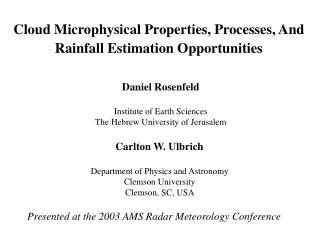
Cloud Microphysical Properties, Processes, And Rainfall Estimation Opportunities Daniel Rosenfeld Institute of Earth Sciences The Hebrew University of Jerusalem Carlton W. Ulbrich Department of Physics and Astronomy Clemson University Clemson, SC, USA

E N D
Cloud Microphysical Properties, Processes, And Rainfall Estimation Opportunities Daniel Rosenfeld Institute of Earth Sciences The Hebrew University of Jerusalem Carlton W. Ulbrich Department of Physics and Astronomy Clemson University Clemson, SC, USA Presented at the 2003 AMS Radar Meteorology Conference
In the beginning (1947) Marshall and Palmer created the MP Drop Size Distribution And MP Z-R relationship
and more… and more…
Early classification of Z-R by rainfall types Fujiwara, 1965: Thunderstorms Z = ARb A Rain Showers Continuous Rain b
Early classification of Z-R by geographical variation Stout and Muller, 1968 A and b of Z-R relations with geographical variation. Muller and Simms, 1966
However, lack of physically based classification created a tower of Babel of Z-R relations The building of the tower of Babel by Pieter Bruegel, 1563 Oil on oak panel, Kunsthistorisches Museum Wien, Vienna
Forms of the raindrop size distribution (RDSD) Exponential: N(D)=N0exp(-3.67D/D0) Marshall-Palmer (1948), Laws-Parsons (1943), Best (1950) Log-Normal: N(D)=N0D-1exp[-cln2(D/Dg)] Levin (1954) Gamma: N(D)=N0Dexp[-(3.67+)D/D0] Deirmendjian (1969), Willis (1984), Ulbrich (1983) Interdependence of RDSD parameters In all of the above the RDSD parameters are NOT independent. Attempts to resolve this problem. Normalized forms: do not remove interdependence Willis (1984), Testud et al. (2001), Chandrasekar and Bringi (1987) New RDSD parameters Haddad et al. (1996): attempt to establish independent parameters. D’=DmR-0.155 s’=smDm-0.2R0.031exp(0.017R0.74) Gamma distribution parameters N0 and ; strong correlation. Chandrasekar and Bringi (1987) In this work the Gamma distribution is used together with Z-R relations to determine RDSD parameters and integral rainfall parameters defined in terms of the RDSD parameters (in spite of lack of independence).
Rain Parameter Diagram of Atlas & Chmela (1957) Exponential RDSD. Isopleths of W, Do, No
Atlas-Chmela RAPAD with sample Z-R relations = Equilibrium raindrop size distribution
Method of using the Gamma distribution with the Z-R law parameters. Any two integral rainfall parameters P and Q; Eliminating D0 yields; Inverting gives; With P=Z and Q=R in Z=ARb, can findand N0from A and b. These can then be used to find coefficients and exponents in theoretical D0-R, NT-R, W-R relations.
Z-R relations used in this work Source No. Z-Rs Description Foote (1966) 2 Mountain thunderstorm in AZ, Filter paper meas. Sims (1964) 1 Thundershowers. Illinois. Joss and Waldvogel (1970) 1 Thunderstorm. 25 days total, Locarno, disdrometer) Petrocchi and Banis (1980) 1 Thunderstorm, Norman, OK (disdrometer) Sauvageot (1994) 1 Tropical squall line. Congo Ulbrich et al. (1999) 1 Ave. of 7 thunderstorms in Arecibo, PR.(disdrometer) Tokay et al. (1995) 2 Tropical. Disdrometer data. Darwin, Australia. Maki et al. (2001) 6 15 squall lines. Disdrometer, Darwin, Australia. Tokay and Short (1996) 2 TOGA COARE data. Kapingamarangi atoll, disdrometer Stout and Mueller (1968) 3 Trade wind showers; Marshall Islands Jorgensen and Willis (1982) 2 Hurricane Frederic, 9/12/79 Ulbrich and Atlas (2001) 2 Tropical storms. PMM analysis, TOGA COARE 2DP data. Fujiwara and Yanase (1968) 3 Filter paper meas. Orographic, slopes of Mt. Fuji. Atlas et al. (1999) 2 TOGA COARE, Kapingamarangi atoll, disdrometer. Blanchard (1953) 1 Orographic rain, windward slopes on Mauna Loa. Only those relations used which involve direct measurements of drop size spectra and for which the environmental conditions are well known. No combinations of instruments (radar-raingages or radar-disdrometer, etc.) were considered.
Rain water content, W [g m-3] as a function of rain drop median mass diameter D0 [cm] and drop concentration NT [m-3] for R=10 and R=30 mm h-1, For all Z-R’s
Processes determining the Rain Drop Size Distribution Wilson and Brandes, 1979:
Processes determining the Rain Drop Size Distribution Coalescence Modification of the DSD by coalescence alone decreases the numbers of small diameter drops and increases those of the larger drops. Consequently D0 must increase and the total number concentration of drops NT must decrease. The process probably also increases , but not by much. The result is a decrease in N0 and a consequent increase in A and small decrease in b. Because of the small change in , we may therefore use the same RAPAD before and after modification. The result is an approximate parallel shift in the Z-R relation on the RAPAD upward and to the left, perpendicular to the D0 isopleths.
Processes determining the Rain Drop Size Distribution Breakup Modification of the DSD by break-up alone increases the numbers of small diameter drops and decreases the numbers of large diameter drops. There must be a consequent decrease in D0 and an increase in NT. Accordingly, N0 must increase. There is probably a small change in with a tendency toward a decrease. The end result is a decrease in A and a small increase (or perhaps no change) in b. Because of the small change in we may use the same RAPAD before and after modification. There is therefore an approximate shift in the Z-R relation on the RAPAD downward and to the right, approximately parallel to the D0 isopleths.
Processes determining the Rain Drop Size Distribution Coalescence And Break-up Combined Break-up is more important at the larger sizes, coalescence more important at small sizes (insofar as numbers are concerned). Both processes acting together increase substantially. This requires using a different RAPAD before and after modification, i.e., the isopleths will shift. The apparent increase in will decrease b. What will happen to A depends on which of the two processes in predominant.
Processes determining the Rain Drop Size Distribution Accretion Since accretion of cloud particles by raindrops acts to increase the sizes of all particles without increasing their numbers, then NT must remain unchanged. There is probably a shift of the DSD parallel to itself to larger diameters with a consequent increase in D0. Since NT remains constant N0 must decrease. The result is an increase in A and probably little change in b. Since is unchanged the same RAPAD before and after modification can be used. Therefore, the Z-R law will be shifted parallel to itself upward on the RAPAD.
Processes determining the Rain Drop Size Distribution Evaporation The presence of evaporation will result in a greater loss of the numbers of small diameter particles than large drops. Consequently, NT is not constant and must decrease. There must also be a substantial change in the shape of the DSD so that increases. Also, D0 must increase. The result is a decrease in N0 and an increase in A. In addition, since increases, b must decrease. Since there is a change in it is necessary to use a different RAPAD before and after modification.
Processes determining the Rain Drop Size Distribution Updraft The presence of an updraft eliminates the smallest particles from the DSD at the lower levels. The effect on the DSD is therefore the same as evaporation. .
Processes determining the Rain Drop Size Distribution Downdraft Here we assume that the downdraft is accelerating downward. There will therefore be an increased flux of small particles thereby decreasing which means b must increase. Also, NT must increase and D0 decrease. Hence N0 must increase which results in a decrease in A. Because of the change in it is necessary to use a different RAPAD before and after modification.
Processes determining the Rain Drop Size Distribution Size-sorting Size sorting tends to make the DSD much narrower which means must increase substantially. Therefore b must decrease. NT must obviously decrease, but what happens to D0 depends on which segment of the precipitation streamer is being observed. So A would either increase or decrease depending on what happens to D0. It is likely that the decrease in NT will dominate the change in D0 so that A would increase, but this is not certain. Because of the dramatic change in a different RAPAD would definitely have to be used before and after modification.
Processes determining the Rain Drop Size Distribution Equilibrium DSD: Z = 600 R; D0 = 1.75 mm Hu and Srivastava (1995)
Impact of Cloud DSD on the evolution of Rain DSD • Maritime Cloud DSD • Cloud drop coalescenceDrizzle • Drizzle coalescence Raindrops • More coalescence larger raindrops • breakup and equilibrium DSD • Approaching D0e from below • Continental Cloud DSD • Cloud drop accretiongraupel • haillarge raindrops • breakup • equilibrium DSD • Approaching D0e from above
Equilibrium Maritime Continental Trends of D0 for convective maritime and continental clouds. Rain water content, W [g m-3] as a function of rain drop median mass diameter D0 [cm] and drop concentration NT [m-3] for R=30 mm h-1, For all Z-R’s.
The classification scheme of convective clouds into microphysical zones according to the shape of the temperature – effective radius relations Note that in extremely continental clouds re at cloud base is very small, the coalescence zone vanishes, mixed phase zone starts at T<-15oC, and the glaciation can occur at the most extreme situation at the height of homogeneous freezing temperature of –39oC. In contrast, maritime clouds start with large re at their base, crossing the precipitation threshold of 14 mm short distance above the base. The deep rainout zone is indicative of fully developed warm rain processes in the maritime clouds. The large droplets freeze at relatively high temperatures, resulting in a shallow mixed phase zone and a glaciation temperature reached near –10oC Rosenfeld and Lensky, 1998
Why is Continental - Maritime classification so fundamental? Annual average lightning density [flashes km-2] Lightning prevail mostly over land, whereas rainfall is similar over land and ocean, indicates fundamental differences between continental and maritime rainfall.
Differences in rain DSD forming processes between Maritime and Continental Clouds: In Maritime clouds there are: More Coalescence Rainout D0 < D0e Smaller R(Z) Lower updrafts Smaller D0 Smaller R(Z) Less evaporation Smaller D0 Smaller R(Z) In Continental clouds there are: Less Coalescence No Drizzle No small rain drops Hydrometeors start as graupel and hail D0 > D0e Larger R(Z) Larger updrafts Larger D0 Larger R(Z) More evaporation Larger D0 Larger R(Z) .
Disdrometer measured DSD of continental and maritime rainfall, as micophysically classified by VIRS overpass. The DSD is averaged for the rainfall during +- 18 hours of the overpass time. The disdrometers are in Florida (Teflun B),Amazon (LBA),India (Madras) and Kwajalein. Application of TRMM Z-R shows a near unity bias in maritime clouds, but overestimates by a factor of 2 rainfall from continental clouds. Rosenfeld and Tokay, 2002
a & b in Ze = 10^a R^b Ze-R relations in Gadanki SW NE SW NE Rain Obs in Asia for PR Algorithm Tuning Study items: DSD, BB model, BB & RR comp. with PR. One of the Major Findings:DSD properties: Significant seasonal dependence in India: Large D0 in SW monsoon,low D0 in NE. Not much seasonal dependence in Singapore. By T. Kozu Kozu
Z-R relations for rainfall from maritime and continental convective clouds. The rain intensities for 40 and 50 dBZ are plotted in the figure. Note the systematic increase of R for a given Z for the transition from continental to maritime clouds. 1. Arizona mountain thunderstorms (Foote 1966) 646 1.46 3. Swiss Locarno thunderstorms, continental (Joss and Waldvogel , 1970) 830 1.50 4. Illinois thunderstorms, continental (Sims, 1964) 446 1.43 5. Oklahoma thunderstorms, moderate continental (Petrocchi and Banis, 1980) 316 1.36 6. Congo Squall line. Tropical continental (Sauvageot, 1994) 425 1.29 7. PurtoRico thunderstorms. Coastal, moderate maritime (Ulbrich et al., 1999). 261 1.43 8. Darwin Squalls. Coastal, tropical maritime (Maki et al., 2001) 232 1.38 9. Darwin Convective DSD. Coastal, tropical maritime (Tokay et al., 1995) 175 1.37 10. COARE Convective DSD. Equatorial maritime (Tokay and Short, 1996). 139 1.43 11. Marshall Trade wind cumulus. Warm rain maritime (Stout and Mueller, 1968) 126 1.47 12. Marshall Showers. Equatorial maritime. (Stout and Mueller, 1968) 146 1.42 E. Equilibrium DSD. 600 1.00
The variation of D0 with the liquid water content (W) and total drop concentration (NT) for R=10 and 30 mm hr-1 of convective rainfall in maritime and continental regimes. Note that D0 decreases from continental to maritime clouds.
ConvectiveStratiform classification In Maritime Convective clouds : More Coalescence Rainout D0 < D0e Smaller R(Z) Less evaporation Smaller D0 Smaller R(Z) In Stratiform clouds : Aggregation of ice Larger D0 Larger R(Z) More evaporation Larger D0 Larger R(Z) .
Tropical Convective – Stratiform received much attention because of different vertical profiles of latent heating, to which the global circulation is quite sensitive. Convective R(Z)almost double than Stratiform R(Z). [Tokay and Short (1995, 1996); Atlas et al. (2000); Ulbrich and Atlas (2001) ] C/S classification already applied to TRMM Z-R
Z-R relations for rainfall from tropical convective and stratiform clouds. The rain intensities for 30 and 40 dBZ are plotted in the figure. Note the systematic decrease of R for a given Z for the transition from convective to stratiform clouds. 1. Darwin Convective DSD. Coastal, tropical maritime (Tokay et al., 1995) 175 1.37 a. Darwin Stratiform DSD. Coastal, tropical maritime (Tokay et al., 1995) 335 1.37 2. Marshall Showers. Equatorial maritime. (Stout and Mueller, 1968) 146 1.42 b. Marshall continuous. Equatorial maritime. (Stout and Mueller, 1968) 226 1.46 3. COARE Convective DSD. Equatorial maritime (Tokay and Short, 1996). 139 1.43 c. COARE Stratiform DSD. Equatorial maritime (Tokay and Short, 1996). 367 1.30 4. COARE Convective aloft, by updraft (Ulbrich and Atlas, 2001) 120 1.43 d. COARE Stratiform aloft, by updraft (Ulbrich and Atlas, 2001) 203 1.46 5. Hurricane eye wall. (Jorgensen and Willis, 1982) 287 1.27 e. Hurricane rain bands. (Jorgensen and Willis, 1982) 301 1.38 E. Equilibrium DSD. 600 1.00
The variation of D0 with the liquid water content (W) and total drop concentration (NT) for R=10 and R=30 mm hr-1 of convective rainfall in maritime and continental regimes. Note that D0 increases from convective to stratiform clouds. Note that Hurricane has near equilibrium D0
In orographic clouds with active coalescence: Early fall to the mountain slope of small hydrometeors Highly immature DSD D0 << D0e Much Smaller R(Z) .
Z-R relations for rainfall from maritime orographic clouds. The rain intensities for 30 and 40 dBZ are plotted in the figure. Note the systematic increase of R for a given Z for greater orographic uplifting. 1. Mount Fuji, at height of 1300 m. (Fujiwara and Yanase, 1968) 240 1.48 2. Mount Fuji, at height of 2100 m. (Fujiwara and Yanase, 1968) 88 1.28 3. Mount Fuji, at height of 3400 m. (Fujiwara and Yanase, 1968) 48 1.11 a. Marshall Trade wind cumulus, 0 m. (Stout and Mueller, 1968) 126 1.47 b. Hawaii, Mauna Loa, 800 m. (Blanchard., 1953) 31 1.71 E. Equilibrium DSD. 600 1.00
The variation of D0 with the liquid water content (W) and total drop concentration (NT) for R=10 and R=30 mm hr-1 of orographic rainfall in maritime clouds. Note that D0 decreases substantially with the orographic uplifting.
Summary: All Z-R classifications combined The variation of D0 with the liquid water content (W) and total drop concentration (NT) for R=10 and 30 mm hr-1 of convective rainfall in maritime and continental regimes.
Summary A review of Z-R relations based on cloud physics RDSD forming processes revealed that Z-R behave systematically, Producing larger R for the same Z when going from: Continental Maritime (X4) Maritime Orographic (X4) Stratiform Convective Maritime (X2) Opportunities Classification criteria can be detected by: Satellite (cloud drop effective radius for continentality); Radar 3-D structure; Dynamics of orographic lifting. Potential for dynamic Z-R for space and ground based radars, accounting for systematic biases by factors of 2 to 4.