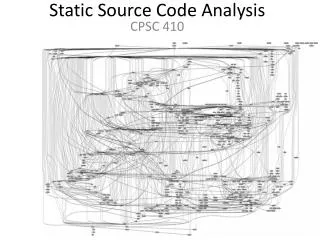
Static Source Code Analysis

1. Static Source Code Analysis CPSC 410

2. Static Analysis • Want to determine execution properties of source code 1. Without executing all possible test cases 2. Without reverse-engineering it in our head • Execution properties • Properties that do not depend on the structure • Properties that are invariant over Refactoring

3. Static Analysis Overview • Provides • Automated Abstract Reasoning • Uses • Dataflow analysis over Control Flow Graphs • Abstract program Operations • Branch Predicate analysis

4. Abstract Reasoning • Asks questions about program variable properties without executing the program. • Example: Does the value from input( ) affect the value of the variable x? y = input ( ); z = y + 5; y = 6; x = z;

5. Abstract Reasoning Examples • If a program takes no negative inputs, has no negative constants, uses no subtraction or bit operators, … • It won’t have a negative output • If a program initializes all variables when they are declared • It won’t have a null pointer exception • A variable in an if-branch, when not assigned-to in the branch • can’t have a value that contradicts the if-condition

6. Dataflow Motivation • Determine the paths that data follows so that we can apply abstract reasoning at a fine granularity Example • If we know foo uses no negative numbers • and bar is only called by foo bar(x) { …sqrt(x); }

7. Abstract Operator Motivation • Interpret program operators on variable properties instead of values • Addition examples Pos + Pos = Pos Neg + Neg = Neg Pos + Neg = ? ? + Pos = ? • Multiplication examples Pos * Pos = Pos Neg * Neg = Pos Pos * Neg = Neg Pos * ? = ?

8. Branch Analysis Motivation if(y < 0) { throw new IllegalArgumentException(); } if(x > y) { z = x * -1; } else { z = 1; } Can z be negative at the of this code?

9. Data-flow Requires Control-flow Graph Can base analysis on a model of the control-flow of the program A node in a control-flow graph (CFG) represents a statement An edge (i,j) represents a possible transfer of control from node i to node j • Consider Single Method CFG • Ignoring Exceptions

10. Single Method Control-Flow • Use two special nodes to denote entry and exit of method Start points to first statement all return statements point to Exit • Connect with other nodes for method body • Assignments • Declarations • Conditionals/Loops/Logical Operators • Input/Output Start Exit

11. Statements • Use Statement Level for Dataflow Analysis • Not Block Level! Example (in red): a = b if ( a > b ) {a = b; x = x + 1;} print(x); x = x + 1 a = b x = x + 1

12. Conditional Conditionals have outgoing arcs labeled true or false a > b true a = b Example: false if ( a > b ) { a = b; x = x + 1;} print(x); x = x + 1 print(x)

13. Loop Last statement in loop has a back edge to loop condition x > y true while (x > y) { x = x + 1; y = y * 2; } return y; x = x + 1 false y = y * 2 return y;

14. Method Start int method(int a, int b, int x, int y) { if ( a > b ) { a = b; x = x + 1; } print(x); while (x > y) { x = x + 1; y = y * 2; } return y; } a > b true x > y a = b true false x = x + 1 false x = x + 1 print(x) y = y * 2 return y; Exit

15. Iterative Data-Flow Analysis • Iterative Data-Flow Analysis Framework • Theoretical framework for many dataflow analyses • Iterates over CFG and annotates nodes/edges with sets of assertions • Each analysis chooses: 1. Domain 2. Approximation 3. Direction 4. Transfer functions for each CFG node type • Examples • Liveness • Available Expressions • Reaching Definitions • Information flow security

16. Data-Flow Analysis Framework • Domain • What kind of solution is the analysis looking for? • Ex. Variables have not yet been defined • Algorithm assigns a set of assertions to each node/edge • Approximation • Useful data-flow properties are never 100% accurate • Rice’s Theorem, from 1953 • Lower approximation is called a MUST analysis • Set of solutions found is smaller than the set of actual solutions • Upper approximation is called a MAY analysis • Set of solutions found may be larger than the set of actual solutions

17. Data-Flow Analysis Framework • Direction • Forwards: For each node/edge, computes information about past behavior • Backwards: For each node/edge, computes information about future behavior • Transfer Functions • JOIN: Specifies how information from adjacent nodes /edges is propagated • MAY: Union of adjacent edges • MUST: Intersection of adjacent edges • GEN: Specifies which possible solutions are generated at the node/edge • KILL: Specifies which possible solutions are removed at that node/edge

18. Data-Flow Algorithm • Start at the top (bottom) of the CFG • Forwards: top • Backwards: bottom • At each node compute: (JOIN() – KILL(node)) U GEN(node) At each branch: Follow all paths, in any order, up to node where path merges Once all paths up to merge are complete, continue at merge node • If all JOIN edges are not yet computed, • use empty set (MAY) • universal set (MUST) • For loops: • repeat until the solution for all nodes in loop doesn’t change • Called the “fixed-point”

19. Liveness • A variable is live at a node if its current value can be read during the remaining execution of the program • i.e. it holds a value needed in the future. • Domain: program variables • Backwards MAY analysis

20. Liveness Example

21. Liveness Transfer Functions • Exit • GEN(exit) = { } • KILL(exit) = { } • Conditions and Output • GEN(stmt) = Set of all variables appearing in the statement • KILL(stmt) = { } • Assignment • GEN(assignment) = Set of all variables appearing on the right-hand side • KILL(assignment) = Set with variable being assigned to • Declaration • GEN(declaration) = { } • KILL(declaration) = Set of variables being declared • Other • GEN(other) = { } • KILL(other) = { }

22. Liveness Example {x, y} {x} {x, y} { } {x} true false { } {x} {x, z} {x, z} START true false {x, z} { x } { } END

23. Liveness Application • Memory Allocation • Since y and z are never live at the same time, they can share the same memory location • Performance Optimization • Assignment, z = z – 1, is never used

24. Data-Flow Framework Summary • Generic framework for different analyses • Each analysis defines • Domain • Approximation • Direction • Transfer Functions • Used for optimization, verification, and testing