Download
1 / 25
250 likes | 380 Views
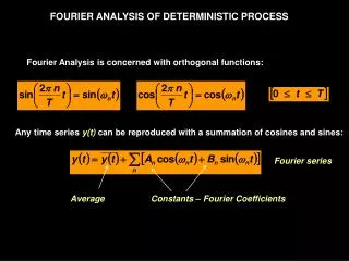
Fourier Analysis of Systems. Ch.5 Kamen and Heck. 5.1 Fourier Analysis of Continuous-Time Systems. Consider a linear time-invariant continuous-time system with impulse response h(t). y(t) = h(t) * x(t)

E N D
Fourier Analysis of Systems Ch.5 Kamen and Heck
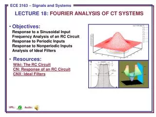
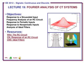
5.1 Fourier Analysis of Continuous-Time Systems • Consider a linear time-invariant continuous-time system with impulse response h(t). • y(t) = h(t) * x(t) • In this chapter the system is not necessarily causal, but the impulse response is absolutely integrable—this is a stability condition.
5.1 Fourier Analysis of Continuous-Time Systems (p.2) • Assume that the Fourier transform of h(t) exists and is given by H(). • From the results of chapter 3: • Y()= H() X(). (Eq. 5.4) • Also we have: • |Y()|= |H()||X()|. • Y()= H() + X().
5.1.1 Response to a Sinusoidal Input • Let x(t) = A cos(0t + ), for all t. • From Table 3.2, X() = A[e -j ( + 0 ) + e j ( - 0 ) ] • Now H() ( + c) = H(-c) ( + c) • And so we have: Y()= H() X() = AH()[e -j ( + 0 ) + e j ( - 0 ) ] = A[H(-0 )e -j( + 0) +H(0 )e j(0-0)]
5.1.1 Response to a Sinusoidal Input (p.2) • Also, h(t) is real valued and so |H(-0)| = |H(0)| H(-0) = - H(0) (Eq. 5.9) • This then gives the Fourier transform of the output to be Y() = A |H(0)| [e –j(+ H(0))( + 0) +e j(+ H(0))(0-0)] (Eq. 5.10) • From the Table of inverse transforms: y(t) = A |H(0)| cos(0t + + H(0) )
Example 5.1 Response to Sinusoidal Inputs • Let the frequency response function be given by a magnitude function and phase function: • |H()| = 1.5 for 0 20 and 0 for >20 • H() = - 60 for all . • If the input is: • x(t) = 2 cos(10t + 90) + 5cos(25t + 120) for all t. • Then the output is: • y(t) = 3 cos(10t + 30) for all t.
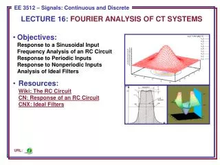
Example 5.2 Frequency Analysis of an RC Circuit • See Figure 5.1. • Figure 5.2 and Figure 5.3 show results.
Example 5.3 Mass-Spring –Damper System • Section 1.4, Figure 1.25. • M y’’(t) + D y’(t) + K y(t) = x(t) (5.23) • M is the mass. • D is the damping constant. • K is the stiffness constant. • x(t) is the force applied to the mass. • y(t) is the displacement of the mass relative to the equilibrium position.
Example 5.3 (cont.) • Take the Fourier transform of both sides of the differential equation: • M(j)2Y() + D(j)Y()+ KY() = X() • Y()(M(j)2+ D(j)+ K) = X() • Y()= X() / [(M(j)2+ D(j)+ K)] • Y()= H() X() • where H()= 1/(M(j)2+ D(j)+ K)
5.2 Response to Periodic and Nonperiodic Inputs • Periodic Inputs • x(t) = a0 + k=1, Ak cos(k0t +k) for all t • y(t) =H(0) a0 + k=1,|H(k 0)|Ak cos(k0t +k + H(k 0)) for all t (Eq. 5.24) • Example 5.4 Response to a Rectangular Pulse Train • Nonperiodic Inputs • y(t) = inverse Fourier Transform of H()X(). • Example 5.5 Response of RC Circuit to a pulse.
5.3 Analysis of Ideal Filters • Figure 5.12 illustrates the magnitudes of 4 ideal filters. • Lowpass • Highpass • Bandpass • Bandstop • More complicated ideal filters can be obtained by cascading the above: • Figure 5.13—Ideal Comb Filter
5.3.1 Phase Functions • To avoid phase distortion, the ideal filter should have linear phase over the passband of the filter. • H() = -td for all in the passband. • td is a fixed positive number that represents a time delay through the filter.
5.3.2 Ideal Linear-Phase Lowpass Filter • H() = e –jtd, -BB, and 0 elsewhere. • The input response can be found by finding the inverse of the frequency response: • Rewrite frequency response: H() = p2Be –jtd • From Table 3.2: (/2) sinc(t/2)p() • Let = 2B, (2B/2) sinc(2Bt/2)p2B() • Apply time shift: • (2B/2) sinc(2B(t-td)/2) p2Be –jtd • Hence: h(t) = (B/) sinc(B(t-td)/) for all t. • For other ideal filters, the analysis is similar.
5.4 Sampling • Let p(t) = n=-, (t-nT) Eq. 5.47 • Then the sampled waveform is • x(t)p(t) = n=-,x(t)(t-nT)=n=-, x(nT)(t-nT) • Determine the Fourier transform of the sampled signal: • Reconsider the pulse waveform: (page 243) • p(t) = k=-,ckejkst , where s = 2/T is the sampling frequency. • Then the Fourier coefficients are ck=1/T
5.4 Sampling (p.2) • Now, xs(t) =x(t)p(t) = k=-,x(t)(1/T)ejkst • Use the property of multiplication by a complex exponential: • x(t)ej0t X( - 0) • Thus, the transform of the sampled signal: • Xs() =k=-,(1/T)X( - kS) • See Figure 5.17 for the case where the spectral replicas do not overlap.
5.4.1 Signal Reconstruction • Suppose that the orignal signal, x(t), is bandlimited: |H()|= 0 for > B. • If the sampling frequency, s 2B, then the replicas in Xs() will not overlap. • Now consider and ideal low-pass filter as shown in Figure 5.18 (page 245). • If the sampled signal is passed through the ideal-low pass filter, the only component passed is X().
Sampling Theorem • A signal with bandwidth B can be reconstructed completely and exactly from the sampled signal xs(t) = x(t)p(t) by lowpass filtering with cutoff frequency B is the sampling frequency if the sampling frequency s is chosen to be greater than or equal to 2B. The minimum sampling frequency is called the Nyquist sampling frequency.
5.4.2 Interpolation Formula • Pages 246 and 247 goes through the formal discussion of passing the sampled signal through an ideal lowpass filter. • The final equation, (5.57), is called the interpolation formula.
5.4.3 Aliasing • If the replicas overlap, reconstruction results with high frequency components being transposed to lower frequency components—this is called aliasing. • Figure 5.20 and 5.21 illustrate the concept. • Example 5.6 and 5.7 discuss sampling of speech. • Note: in the real-world an ideal aliasing filter cannot be built, so there will always be some distortion.
5.5 Fourier Analysis of Discrete-Time Systems • Convolution: y[n] = h[n] * x[n] • Frequency Response: H(Ω) (DTFT of h[n] • Y(Ω) = H(Ω) X(Ω)
5.5.1 Response to a Sinusoidal Input • Let x[n] = A cos(Ωo n + θ), n=0, ±1,±2 … • Take DTFT of x[n]. • Multiply by frequency response. • Take inverse DTFT (see page 250) • y[n] = A ǀH(Ω o)ǀ cos(Ωo n + θ + H(Ωo)) n=0, ±1,±2 …
Example 5.8 Response to a Sinusoidal Input • Let H(Ω) = 1 + e-jΩ • Let x[n] = x1[n] + x2[n] = 2 + 2 sin(π/2 n) • Then H(0) = 1 + 1 = 2 • And H(π/2) = 1 + exp(-jπ/2) = 1 + 0 –j • So, y[n] = 2 + (2) (√2)sin(π/2 n - π/4).
Example 5.9 Moving Average Filter • Let y[n] = (1/N){x[n] + x[n-1]+…+x[n-(N-1)]} • Take DTFT and use time-shift property. • Y(Ω) = (1/N){X(Ω) + X(Ω)e-jΩ +…} • Y(Ω) = (1/N){1 + e-jΩ +…+e-j(N-1)Ω} X(Ω) • So H(Ω) = (1/N){1 + e-jΩ +…+e-j(N-1)Ω} • And H(Ω) = {sin(NΩ/2)/N sin(Ω/2)}e-j(N-1)Ω/2 • Figure 5.22 shows frequency response for N=2.
5.6 Application to Lowpass Digital Filtering • 5.6.1 Analysis of Ideal Lowpass Digital Filter • See Figure 5.23 (phase =0) • Let x[n] = A cos(Ωon), n=0,±1,±2,… • Then y[n] = A cos(Ωon), n=0,±1,±2,… for 0≤ Ωo≤B and 0 elsewhere.
5.6.2 Digital-Filter Realization of Ideal Analog Lowpass Filter • Let x(t) = A cos(ωot), -∞≤t ≤∞ • Sample the signal: x[n] = A cos(Ωon) where Ωo = ωoT and t = nT. • For the ideal filter we must have Ωo <π or ωo<π/T. • An analog signal can then be generated from the sampled output. • For this filter, h[n] = (B/π) sinc(Bn/π)