Download
1 / 26
260 likes | 356 Views
Theoretical Aspects of Dark Energy. Matts Roos University of Helsinki Department of Physical Sciences and Department of Astronomy This talk, presented in Tõravere, is an abbreviated version of a review, therefore the section numbering appears a bit disorderly. TexPoint fonts used in EMF.

E N D
Theoretical Aspects of Dark Energy Matts Roos University of Helsinki Department of Physical Sciences and Department of Astronomy This talk, presented in Tõravere, is an abbreviated version of a review, therefore the section numbering appears a bit disorderly. TexPoint fonts used in EMF. Read the TexPoint manual before you delete this box.: AAAAAAAAAAAAA
Contents • Basic theoretical assumptions • Scalar fields • Modified gravity • Exotic models • Conclusions
The Universe is homogeneous on a very large scale. Maybe so, but only within our horizon. Inhomogeneities may appear later when the horizon expands to reveal what is now outside Imagine that we are at the center of a low-density isotropic universe, surrounded by a high-density universe. Both regions decelerate, but the inner region expands faster. Then we would observe an apparentpositive average acceleration. I. Basic theoretical assumptions leading to the background model and the concordance model
2. The Universe is isotropic. We live ina 3+1-dimensional manifold. The metric is that of Robertson and Walker (RW) Limits to an early violation of rotational invariance have been studied, but this cannot be used to explain an accelerated expansion. This leaves ample room for modifications to higher manifolds. a(t) can be modified. Note that flatness impliesk = 0. basic theoretical assumptions continued
basic theoretical assumptions continued • The geometry of space-time is described by Einstein’s General Relativity (GR) • GR is describes the most general kind of interaction which a massless spin-two particle can have and which is consistent with general principles: special relativity, covariance, equivalence , unitarity, stability. • The Einstein tensorGhas 16 components. Here Rmn is the symmetric Ricci tensor, and R is the spatial curvature (theRicci scalar): • Gmn includes derivatives of the metric tensorgmntolowest orderonly. Higher order derivatives would give unsolvable nonlinear equations. • In tensor notation, any metric (also RW) can be written Extensions and modifications to GR are possible.
T00 is the energy densityr. Tiiare the pressure components pi T0i are the energy flow components in the direction i. Vanish for comoving coordinates . Ti0 are the momentum densities in the direction i. Vanish for comoving coordinates . Ti j are the shear of the pressure p i in the direction j. Vanish in an isotropic Universe. Dark Energy could also be included in T. basic theoretical assumptions continued6. The Stress-Energy Tensor T
basic theoretical assumptions continued 7. The Einstein equation:the geometry of the Universe (on the LHS) depends on its energy content (on the RHS) • where • This simplifies to the two Friedmann equations: one for the energy density rand one for the pressure p (say p=px , choosing py=pz=0). In units of c =h =1 they are They define the background or Friedmann-Robertson-Walker (FRW) model: aUniverse filled with cold, almost pressureless matter:r> 0, p &0, therefore it cannot accelerate.
8. The Equation of State In the Friedmann eqs. we replace by H, and p bythe EOS : If wis constant in time, we can differentiate the first FRW equation with respect to t, and then use the second equation to eliminate dH / dt : We can solve this and the first FRW equation to obtain In a matter-dominated universe In a radiation-dominated universe In the vacuum-energy state Acceleration would correspond to This gives the continuity equation or the energy conservation law. w = 0, rdecreases with time w = 1/3 d:o w= -1, r is constant w < -1/3 basic theoretical assumptions continued
DynamicalLwith w = w (t)L with w = -1 on the LHS of Einstein’s equation is static gravity. • Formulae of the ad hoc forms w = w0 f (w1 , t)are based on no theory, describe e.g. a “decaying cosmological const.” • One successful formula is [Wetterich, Phys. Lett. B 594 (2004) 17] which has two parameters, w0 and b. Advantage: it covers the whole observed z range. • The solid line is a best fit with Wm=0.27, w0 = -1.11, b=0.31, dotted lines mark the 95% CL. Figure from Wu and Yu, Phys. Lett. B 643(2006) 315
Scalar fieldsSee also the review by Copeland et al., hep-th/0603057 • We now assume thatL = 0, turning to other solutions. • The dynamical explanation of the accelerating universe could be an all-permeating fluid, a scalar field in Tmnon the right hand side of the Einstein equation • T must have the same transformation properties as G,thus it is required to obey whereLm contains the energy density of the scalar field as well as the density of matter, r m
Scalar fields Tachyon fields • Special relativity in 4-dimensional spacetime forbids tachyons. • But in higher dimensional spacetimes, tachyons may move in the bulk between our brane and other branes. • The potential may be of the form so that the field has a ground state atj = 1. In a flat FRW background From the Friedmann eqs. Hence accelerated expansion occurs for Note that • When matter is added, Friedmann’s equations have to be modified correspondingly.
Scalar fields Chaplygin gas • Consider the special case of a tachyon field with a constant potentialV(j) = A > 0, so that the EOS is b is a free parameter. • The continuity equation can then be integrated to give (withb=1) (Bis a constant) • This has very interesting asymptotic behavior: • at early times this gas behaves like pressureless dust, like CDM, at late times likeL,causing accelerated expansion. • Problem: when the dust effect disappears but CDM remains, this causes a strong ISW effect & loss of CMB power, thus the model is a poor fit to data (SNe, BAO, WMAP).
Modified gravity 5-dimensional DGP gravity Dvali – Gabadadze - Porrati • Assume that the observable physics occurs on a 4-dimensional brane, embedded in a 5-dimensional bulk universe. • Gravitation occurs everywhere in the brane and bulk, but at late time (now) it gets weaker on the brane, it leaks out into the bulk) present accelerated expansion. • The energy scale Mand time scale tof gravity are (with c =h =1): on the braneMPl and tPl = 1/ MPl, in the bulk M5andt5= 1/ M5 . • Let’s define a cross-over length parameter to be fitted to the time scale of acceleration. • On scales r <<rcthe gravitation is located on the 4-dim. brane, and the potential behaves as 1/r ;on scales r >>rcas 1/r 2. • The DGP version of the Friedmann equation is
When H << rc, the root term vanishes ) the usual Friedmann eq. When H ~ rc or H > rc the root term correction becomes important. In flat space(k = 0), and at late times when this becomes a de Sitter acceleration In the space of the parameters Wk , Wm and a density parameter one can generalize the DGP model as follows: where n defines a parametric family. Modified gravity continued
Basic DGP (n = 1) is a poor fit, n = 2 (LCDM) and n = 3 are good fits when constrained by SNLS, ESSENCE, BAO, and WMAP3 data. n>3 fits are poor, need more parameters (Wk or other).Below is plotted Wc versus Wm(the solid line corresponds to Wk=0).Rydbeck, Fairbairn and Goobar, astro-ph/0701495
A combined Chaplygin-DGP model • Remember that the Chaplygin model has a critical scale rc6= B/A : At early times the Chaplygin gas behaves like pressureless dust, like CDM, at late times likeL. • A similar critical scale exists in the DGP model: • Let’s combine the models, setting rc Chaplygin=rcDGP This implies that we explain the accelerating expansion by Modified Gravity including a Dark Energy field. • Hopefully this cures both the Chaplygin gas and the DGP problems.
In flat space (k = 0) the Friedmann equations are then and One can then set up the continuity equation which contains an rc coming only from the DGP Friedmann equation. When the continuity equation is integrated, also the Chaplygin rc –term enters as an integration constant. The result is an algebraic equation of 2nd order in rj . Some of its properties are: At very large rcthe H/ rc –term in the DGP- Friedmann equation becomes negligible, the rj dynamics is like for Chaplygin gas. The rm dynamics separates from the rj dynamics. At small values of rc , the rj and rm dynamics are both affected by the DGP-modified gravity, rj depends on (ln a)/a terms. the LCDM model is not recovered.
Conclusions The accelerated expansion can be explained in two ways: • As a dark energy fluid in the stress-energy tensor (on the RHS of Einstein’s equation). Then why is L so small? And why do quantum vacuum energies not gravitate? • Or, as dark gravity, an intrinsic spacetime curvature of the vacuum, modifying GR (on the LHS). Is this the infra-red consequence of some quantum gravity principle, which remains to be discovered? 3. The coincidence problem “Why now?” is not solved.
VII. Conclusions continued • No data today or in the foreseeable future will be able to distinguish between Dark Energy and Dark Gravity. Anyexpansion historyH(z) can be reproduced by both. • Some data in the future will be able to distinguish between a staticand a dynamic L. A static L with EOS w = -1 fits all present data well, but that does not prove it is correct. • Perhaps the complexity of the correct theory exceeds our mathematical and calculational capabilities (string landscape, gravity with higher order derivatives, nonlinearities).